7 Dynamic Pricing Algorithms Explained (2026 Guide)
Dynamic pricing algorithms use machine learning, reinforcement learning, and rule-based logic to adjust prices automatically. Learn which algorithm fits your business.
Dynamic pricing algorithms are the mathematical engines that automatically adjust your prices based on market conditions. The algorithm decides whether to raise prices when demand surges, drop prices to clear excess inventory, match competitor price cuts, or hold steady when nothing changes.
If you've booked an airline ticket that cost $200 Tuesday and $450 Friday, an algorithm made that pricing decision by analyzing seats remaining, booking velocity, and historical patterns. When Amazon changes prices on millions of products daily, algorithms evaluate competitor pricing, inventory levels, and conversion rates without human intervention.
But "dynamic pricing algorithm" covers dozens of approaches from simple if-then rules to sophisticated machine learning models that experiment and learn. According to AIMultiple's 2026 research on dynamic pricing algorithms, the three main models are rule-based systems, regression models, and reinforcement learning—each with different complexity, data requirements, and use cases.
This post explains seven dynamic pricing algorithms in order of increasing sophistication, how each works with examples, implementation complexity, when to use each approach, and which industries rely on which algorithms.
How Dynamic Pricing Algorithms Work (General Framework)
Every dynamic pricing algorithm follows the same three-step process regardless of sophistication.
Step 1: Data Collection
The algorithm continuously monitors inputs:
Internal data:
- Current inventory levels and days of supply
- Historical sales volume at different price points
- Cost of goods sold (COGS) and margin targets
- Sales velocity and conversion rates
- Product attributes and catalog data
External data:
- Competitor pricing from web scraping or data feeds
- Market demand signals (search volume, social media mentions)
- Seasonal patterns and promotional calendars
- Economic indicators (commodity prices, exchange rates)
- Event calendars (holidays, weather events, local events)
Customer behavior data:
- Time spent viewing products
- Cart abandonment patterns
- Purchase history and frequency
- Device type, location, referral source
Step 2: Price Calculation
The algorithm processes all this data and calculates the optimal price. This is where algorithms differ dramatically—from simple if-then rules to neural networks that learn patterns humans can't detect.
Step 3: Price Updates
Once calculated, the new price pushes to:
- E-commerce websites and mobile apps
- Point-of-sale systems (retail stores)
- Sales quote systems (B2B distribution)
- Third-party marketplaces (Amazon, eBay, Walmart)
- Digital shelf labels (some retailers)
Update frequency ranges from once daily (airlines) to hundreds of times daily (e-commerce high-velocity products) to every few minutes (ride-sharing).
1. Rule-Based Pricing Algorithms
Rule-based pricing follows fixed if-then logic you define. When condition X happens, take action Y. No machine learning, no predictions—just explicit rules.
How It Works
You define pricing rules based on inventory, competitor prices, demand signals, or time-based factors:
Inventory-based rules:
- If inventory > 60 days of supply, discount 20%
- If inventory < 15 days of supply, increase price 10%
- If product hasn't sold in 90 days, mark down 30%
Competitor-based rules:
- If competitor price drops 5%, match within 1 hour
- If competitor price increases 10%, increase 5%
- Always price 3% below lowest competitor for key items
Time-based rules:
- Friday evening: increase ride prices 1.5x
- Last 7 days before departure: airline prices increase 25%
- Monday 9am-5pm: B2B catalog shows standard pricing
- Monday 5pm-Tuesday 9am: show night/weekend surcharge
Demand-based rules:
- If page views increase 50% in 2 hours, raise price 15%
- If cart adds double average, test 10% price increase
Formula
Rule-based pricing doesn't use complex formulas. The logic is:
IF (condition met) THEN (price adjustment)
ELSE IF (different condition) THEN (different adjustment)
ELSE (default price)
Example Implementation
A $67M fastener distributor implemented these rules:
Slow movers: SKUs with no sales in 120 days get 25% discount automatically Fast movers in stock: SKUs moving 5+ orders/week stay at standard price Fast movers low stock: SKUs moving 5+ orders/week with less than 10 days inventory get 8% price increase Competitor tracking: 200 key SKUs monitored daily, price matches any competitor drop within 24 hours
Results after 6 months:
- Inventory turnover improved from 4.2x to 5.1x
- Margin held steady (didn't drop despite more discounting)
- Sales team stopped manually chasing competitor prices for those 200 SKUs
When to Use Rule-Based Algorithms
Rule-based pricing works best when:
- You have clear, documented pricing logic
- Market conditions are predictable
- You want full control and transparency
- You're implementing dynamic pricing for the first time
- Your sales team needs to explain pricing to customers
- You lack historical data for statistical models
- Implementation speed matters (2-4 weeks vs. 3-6 months for ML)
Limitations
- Can't handle complex interactions between variables
- Doesn't learn from outcomes (if a rule fails, you manually update it)
- Requires constant monitoring and rule adjustments
- Misses patterns in data that statistical models catch
- Rules conflict when multiple conditions trigger simultaneously
2. Regression-Based Pricing Algorithms
Regression models use historical data to predict optimal prices. The algorithm learns relationships between price, demand, and other factors by analyzing past transactions.
How It Works
The algorithm builds a statistical model that predicts demand or profit at different price points:
Demand = Base Demand + (Price × Price Coefficient) + (Competitor Price × Competitor Coefficient) + (Seasonality × Season Coefficient) + (Inventory Level × Inventory Coefficient)
The model trains on historical data to learn coefficients. Once trained, you input current conditions (today's competitor prices, current inventory) and the model predicts demand at different price points. The algorithm selects the price that maximizes profit:
Optimal Price = Price that maximizes (Revenue - Cost) = (Price × Predicted Demand) - (Cost × Predicted Demand)
Example Implementation
A $140M electrical distributor built a regression model for commodity wire and cable products (3,500 SKUs with volatile copper pricing):
Model inputs:
- Copper spot price (London Metal Exchange)
- Distributor's current inventory (days of supply)
- Average competitor price from 5 scraped distributor websites
- Day of week (Tuesday orders are 15% higher than Friday)
- Quantity ordered (volume discount thresholds)
Model training: 18 months of transaction history, 240,000 invoices
Results:
- Model recommended prices within 2% of actual optimal price 73% of the time (validated against holdout data)
- Gross margin improved 1.4% on modeled SKUs vs. manual pricing
- Implementation took 12 weeks (8 weeks data prep, 4 weeks model training and validation)
When to Use Regression-Based Algorithms
Use regression when:
- You have clean historical transaction data (12+ months preferred)
- Demand patterns are relatively stable and predictable
- You can identify clear drivers of demand (price, season, competitor pricing)
- You want explainable pricing (you can see which factors influence recommendations)
- Your data team has basic statistical modeling skills
- You need faster implementation than complex ML (2-3 months vs. 4-6 months)
Limitations
- Assumes linear or simple nonlinear relationships (misses complex patterns)
- Requires stable demand patterns (struggles with rapid market changes)
- Can't learn from experiments (doesn't try prices and adapt like reinforcement learning)
- Breaks down when market structure changes (new competitors, product substitutes)
- Needs periodic retraining as relationships shift
3. Reinforcement Learning Algorithms
Reinforcement learning (RL) algorithms experiment with different prices, observe what happens, and learn optimal pricing strategies through trial and error. According to AIMultiple's research, reinforcement learning aims to achieve the highest rewards by learning from environmental data, analyzing customer demand while accounting for seasonality, competitor prices, and market uncertainty.
How It Works
RL pricing treats dynamic pricing as a Markov Decision Process:
- Observe state: Current demand, inventory, competitor prices, time of day, etc.
- Take action: Set a price (from a range of possible prices)
- Observe reward: Sales volume, revenue, or profit generated
- Learn policy: Update pricing strategy based on whether reward was higher or lower than expected
The algorithm doesn't start with a model of how customers respond to prices. It experiments, measures outcomes, and learns which prices work best in different scenarios.
Common RL Approaches for Pricing
Q-Learning: The algorithm maintains a value function that estimates expected future profit for each price in each state. According to research on Q-learning in retail pricing, Q-learning algorithms have proven convergence properties and work well in discrete pricing environments.
Policy Gradient Methods: The algorithm directly optimizes the pricing policy by adjusting parameters to increase expected return. These methods handle continuous price ranges better than Q-learning.
Contextual Bandits: A simplified RL approach that treats each pricing decision independently (no long-term planning). The algorithm balances exploring new prices (to learn) with exploiting known good prices (to maximize profit). Many e-commerce platforms use contextual bandits because they converge faster than full RL.
Example Implementation
A global e-commerce platform ran RL-based dynamic pricing on 50,000 SKUs for 6 months (as documented in arXiv research on RL for e-commerce pricing):
Setup:
- State space included time of day, day of week, inventory level, recent sales velocity, competitor price position, and user browsing behavior
- Action space was 20 discrete price points per SKU (from -30% to +20% vs. base price)
- Reward function maximized gross profit per transaction
- Algorithm used deep Q-learning with neural network approximation
Results:
- 2.7% lift in gross profit vs. rule-based pricing (statistically significant after controlling for external factors)
- Algorithm learned non-obvious patterns: higher prices on Sundays for certain categories, dynamic responses to competitor moves based on product velocity
- Took 8 weeks for algorithm to stabilize (explore enough to learn good policies)
- Required data science team with ML expertise to tune hyperparameters
When to Use Reinforcement Learning
Use RL pricing when:
- You have high transaction volume (thousands of pricing decisions daily)
- Market dynamics are complex with many interacting factors
- You can tolerate learning period where algorithm experiments (2-3 months)
- You have ML/data science team to implement and monitor
- You operate in fast-moving markets (e-commerce, ride-sharing)
- Your competitors change prices frequently
Limitations
- Requires months of experimentation to learn effective policies
- Black box (can't easily explain why algorithm recommends specific prices)
- Needs significant transaction volume to learn patterns
- Expensive to implement and maintain (data science expertise required)
- Can learn suboptimal strategies if reward function isn't perfectly aligned with business goals
4. Bayesian Pricing Algorithms
Bayesian models handle demand uncertainty by calculating probability distributions instead of point estimates. According to Coralogix's guide to dynamic pricing models, the Bayesian model uses Bayesian inference to estimate probabilities of different demand scenarios given available data, determining the price that maximizes expected revenue based on probabilities.
How It Works
Instead of predicting "demand will be 100 units at $50," a Bayesian model says:
- 20% chance demand is 80-90 units
- 50% chance demand is 90-110 units
- 25% chance demand is 110-130 units
- 5% chance demand is 130+ units
The model calculates expected profit across all scenarios and selects the price that maximizes expected value given uncertainty.
Expected Profit = Sum of (Probability of Scenario × Profit in Scenario) across all scenarios
Example Implementation
An airline uses Bayesian pricing for new routes where historical data is limited:
Prior beliefs: Based on similar routes, the model starts with a probability distribution of likely demand Data collection: As bookings come in, the model updates beliefs using Bayes' theorem Pricing decisions: The model recommends prices that maximize expected revenue given current uncertainty about total demand
Benefits:
- Handles low-data scenarios better than regression (which needs large datasets)
- Quantifies uncertainty explicitly (shows not just price recommendation but confidence level)
- Updates in real-time as each booking provides new information
When to Use Bayesian Algorithms
Use Bayesian pricing when:
- You're launching new products with limited historical data
- Demand is highly uncertain or volatile
- You want to quantify confidence in pricing decisions (not just point estimates)
- You're testing new markets or customer segments
- You have statisticians who understand Bayesian inference
Limitations
- Computationally intensive (calculating probabilities across scenarios)
- Requires expertise in Bayesian statistics to set prior beliefs and interpret results
- More complex to implement than regression or rule-based approaches
- Can be overkill for stable, predictable markets where regression works fine
5. Decision Tree Pricing Algorithms
Decision trees use hierarchical if-then rules learned from data. According to research, decision tree models offer a transparent approach to pricing decisions through a series of if-then rules.
How It Works
The algorithm analyzes historical data and builds a tree of decisions:
IF inventory > 45 days:
  IF competitor price > $50:
    Price = $48 (undercut competitor)
  ELSE:
    Price = $45 (discount to move inventory)
ELSE IF inventory 15-45 days:
  IF demand velocity high:
    Price = $55 (standard price, product moving)
  ELSE:
    Price = $52 (slight discount to maintain velocity)
ELSE (inventory < 15 days):
  Price = $58 (premium for scarcity)
Unlike rule-based pricing where you manually define rules, decision trees learn the rules from data. The algorithm finds the splits that best predict optimal pricing.
Example Implementation
A $95M industrial supply distributor used decision trees for pricing 12,000 MRO SKUs:
Training data: 2 years of transactions (1.2M invoices) with features including inventory level, customer segment, order quantity, time since last purchase, competitor price data
Model output: A decision tree with 47 terminal nodes (leaf rules) that recommend prices based on combinations of factors
Results:
- More interpretable than regression (sales team could see logic behind each price)
- Captured nonlinear patterns (e.g., high-volume customers less price-sensitive than expected for certain categories)
- Margin improved 0.9% vs. manual pricing rules
When to Use Decision Trees
Use decision tree pricing when:
- You want interpretable, explainable pricing (can show exact logic to sales teams and customers)
- You have enough data to train a model but want simpler implementation than deep learning
- Your pricing logic has clear thresholds (e.g., inventory levels trigger different strategies)
- You're transitioning from manual rule-based pricing to data-driven approaches
- Regulatory or compliance requirements demand transparency
Limitations
- Can overfit to training data (creates overly specific rules that don't generalize)
- Misses smooth transitions (predicts discrete price jumps at thresholds)
- Less powerful than ensemble methods or neural networks for complex patterns
- Needs periodic retraining as market conditions shift
6. Time Series Forecasting Algorithms
Time series algorithms predict future demand and recommend prices based on historical patterns, seasonality, and trends. According to research on machine learning pricing methods, techniques such as ARIMA (autoregressive integrated moving average) and exponential smoothing capture seasonality, trends, and patterns in pricing and demand data.
How It Works
The algorithm decomposes historical sales data into:
- Trend: Long-term increase or decrease in demand
- Seasonality: Recurring patterns (weekly, monthly, quarterly cycles)
- Cyclical patterns: Longer-term fluctuations tied to business cycles
- Residual variation: Random noise
The model forecasts future demand, then recommends prices that optimize revenue given predicted demand.
When to Use Time Series Pricing
Use time series forecasting when:
- Your products have strong seasonal or cyclical patterns
- Historical demand patterns are relatively stable
- You're planning promotional pricing weeks or months in advance
- You have multi-year historical data
- Lead times require advance pricing decisions (catalogs, contracts)
Limitations
- Assumes future patterns resemble past (breaks down during market disruptions)
- Doesn't account for competitor actions
- Forecasts degrade quickly in fast-changing markets
- Needs manual intervention when structural changes occur
7. Deep Learning Pricing Algorithms
Deep learning uses neural networks with multiple layers to find complex patterns in data. These models handle high-dimensional state spaces (hundreds of input variables) and can learn intricate relationships that simpler algorithms miss.
How It Works
A deep neural network takes inputs (price, inventory, competitor prices, customer features, time features, external data) and processes them through multiple layers of artificial neurons. Each layer learns increasingly abstract representations. The final layer outputs a pricing recommendation or demand prediction.
According to research on deep reinforcement learning for pricing, deep learning approaches gained prominence in applications involving high-dimensional state spaces or continuous pricing variables where traditional methods struggle.
Example Implementation
A major online retailer implemented deep Q-learning for dynamic pricing:
Network architecture: 4-layer neural network with 256 neurons per layer Inputs: 87 features including product attributes, customer browsing history, competitor pricing, inventory, time features, external signals Output: Q-values for 50 possible price points
Results:
- 3.2% improvement in gross profit vs. rule-based pricing
- Model learned interactions between features that regression missed (e.g., how customer browsing duration + time of day + inventory level interact to predict conversion at different prices)
- Required 6 months to implement (data pipeline, model training, production deployment, monitoring)
When to Use Deep Learning
Use deep learning pricing when:
- You have massive datasets (millions of transactions)
- Your problem has high-dimensional complexity (dozens of relevant features)
- Simpler models have plateaued in performance
- You have ML engineering team with deep learning expertise
- You can invest 6-12 months in development
- Transaction volume justifies the investment (high-frequency pricing for large catalogs)
Limitations
- Extreme complexity (requires specialized expertise)
- Black box (nearly impossible to interpret why specific prices recommended)
- Requires enormous datasets to train effectively
- Expensive to implement and maintain
- Risk of overfitting if not carefully validated
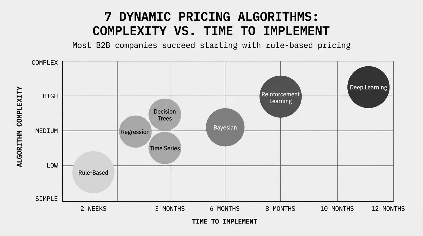
Algorithm Comparison: Which Should You Use?
| Algorithm | Complexity | Data Required | Time to Implement | Best For | Avoid When |
|---|---|---|---|---|---|
| Rule-based | Low | Minimal | 2-4 weeks | Clear pricing logic, first implementation, need explainability | Market is complex with many interacting factors |
| Regression | Medium | 12+ months | 2-3 months | Stable demand, clean data, want explainable model | Demand is chaotic or nonlinear |
| Reinforcement Learning | High | High volume needed | 4-6 months | Complex markets, high transaction volume, can tolerate learning period | Low volume, need immediate results, lack ML expertise |
| Bayesian | Medium-High | Works with limited data | 3-4 months | High uncertainty, new products, want confidence intervals | Stable market where regression works fine |
| Decision Trees | Medium | 12+ months | 2-3 months | Need transparency, nonlinear patterns, transitioning from manual rules | Very high-dimensional problems |
| Time Series | Medium | 2+ years | 2-3 months | Strong seasonality, advance planning, catalog pricing | Fast-changing competitive markets |
| Deep Learning | Very High | Millions of records | 6-12 months | Massive scale, high-dimensional, other methods plateaued | Small-medium business, lack ML team |
Dynamic Pricing Algorithms in Practice: Industry Breakdown
Airlines: Primarily use regression models with time series forecasting. Prices update 1-2 times daily based on seats remaining, booking velocity, and historical patterns. Some airlines layer RL for specific routes.
E-commerce (Amazon, Walmart): Mix of rule-based (for long-tail products), regression (for high-volume staples), and reinforcement learning (for competitive categories). Prices update hundreds of times daily for high-velocity SKUs.
Ride-sharing (Uber, Lyft): Surge pricing uses simplified RL (contextual bandits) that responds to supply-demand imbalances in real-time. Updates every few minutes.
Hotels: Time series forecasting for advance bookings, rule-based pricing for last-minute inventory. Prices update multiple times daily.
B2B Distribution: Most use rule-based pricing with manual overrides. The few implementing ML typically start with regression for commodity products with volatile costs. Weekly or monthly price updates, not real-time.
Getting Started: The Practical Path
Most companies succeed by starting simple and layering sophistication:
Phase 1 (Months 1-3): Implement rule-based pricing for 200-500 SKUs. Learn what data you need, test with sales team, validate results.
Phase 2 (Months 4-9): Add regression models for high-volume products with clean demand patterns. Compare regression recommendations to rule-based pricing and measure lift.
Phase 3 (Months 10-18): Consider reinforcement learning for complex categories if regression plateaus. Requires hiring or training ML expertise.
Common mistake: Starting with complex ML before mastering rule-based pricing. You waste months building infrastructure and models before understanding whether dynamic pricing fits your business at all.
For more on when dynamic pricing makes sense for B2B companies and implementation strategy, see our complete dynamic pricing guide.
Sources
- AIMultiple: Dynamic Pricing Algorithms in 2026: Top 3 Models
- Coralogix: Dynamic Pricing Models: Types, Algorithms, and Best Practices
- arXiv: Dynamic Retail Pricing via Q-Learning - A Reinforcement Learning Framework
- arXiv: Dynamic Pricing on E-commerce Platform with Deep Reinforcement Learning: A Field Experiment
- Flipkart Commerce Cloud: How Dynamic Pricing Solution Leverage Machine Learning
Last updated: February 24, 2026
Frequently Asked Questions
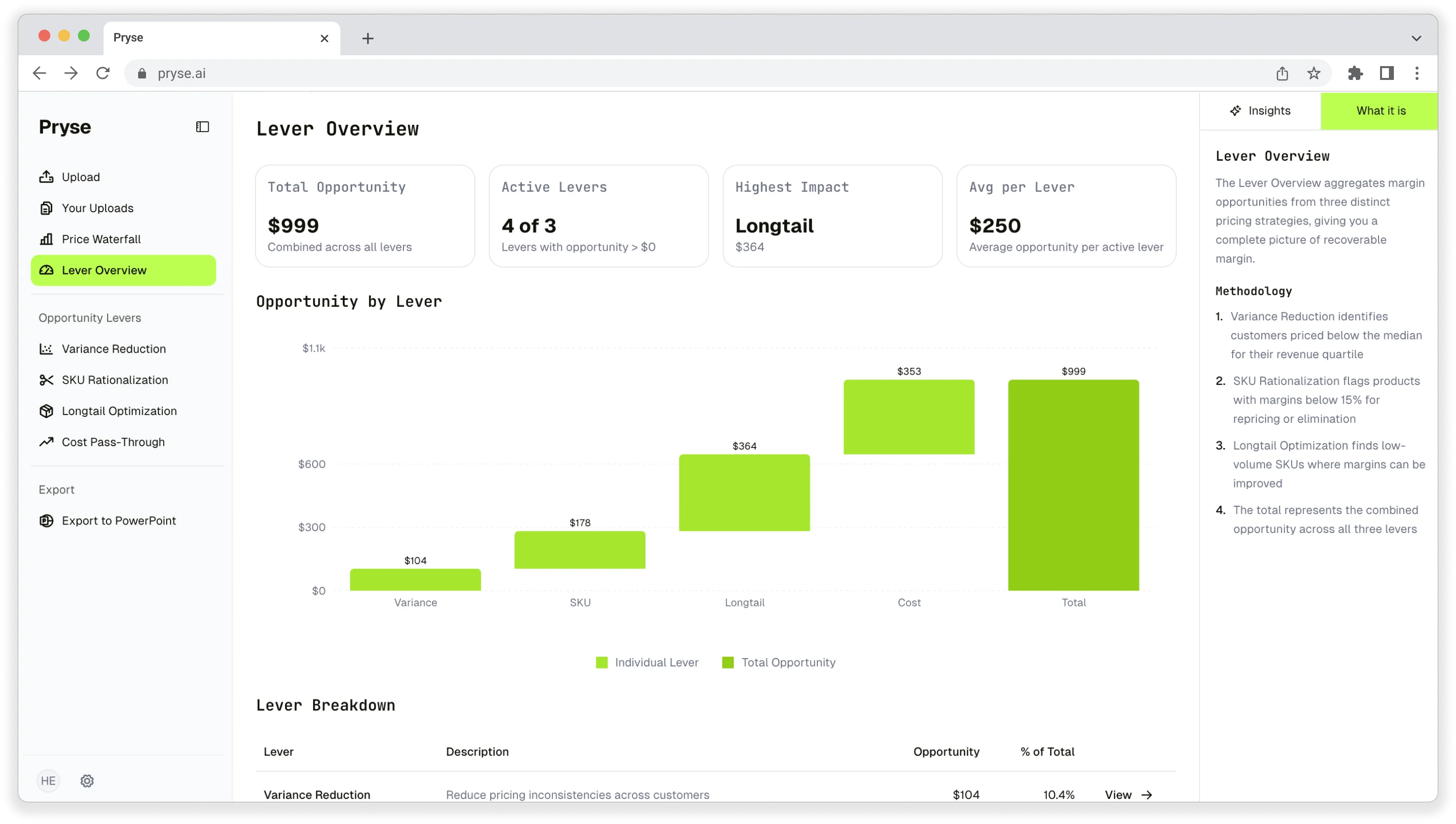
Want to analyze your entire product catalog?
Pryse automatically identifies margin leakage across thousands of SKUs. Upload your data and find hidden profit in 24 hours.
One-time $1,499 diagnostic. No subscription required.