What is the price elasticity formula?

The basic price elasticity formula is: PED = (% Change in Quantity Demanded) / (% Change in Price). It measures how much demand changes when you change price. A result of -2.0 means a 1% price increase causes a 2% drop in quantity demanded.

What's the difference between the basic formula and midpoint method?

The basic formula calculates percentage changes from the starting values. The midpoint method uses the average of starting and ending values, giving the same result whether price increases or decreases. Use the midpoint method for accuracy when analyzing price changes after they happen.

How do you calculate price elasticity step by step?

Calculate the percentage change in quantity: (New Quantity - Old Quantity) / Old Quantity. Calculate percentage change in price: (New Price - Old Price) / Old Price. Divide the quantity change percentage by the price change percentage. The result is your price elasticity coefficient.

What does a price elasticity of -0.5 mean?

A coefficient of -0.5 means demand is inelastic. A 10% price increase will decrease quantity demanded by only 5%. Products with inelastic demand can handle price increases without losing significant volume. Essential B2B supplies often have inelastic demand.

What is elastic vs inelastic demand?

Elastic demand means the coefficient is less than -1 (like -2.5). Customers are sensitive to price changes. Inelastic demand means the coefficient is between 0 and -1 (like -0.4). Customers are less sensitive to price. Commodity products tend to be elastic. Specialty or mission-critical items tend to be inelastic.

Can you measure price elasticity in B2B?

Yes, but it's harder than in B2C. You need sufficient transaction data across different price points. Segment customers by size, industry, or region and calculate elasticity within each segment. B2B elasticity varies more by customer segment than consumer markets due to different value perceptions.

Why use the midpoint method instead of the basic formula?

The midpoint method gives consistent results regardless of direction. If price goes from $10 to $12, then back to $10, the basic formula gives different elasticity coefficients for each change. The midpoint method gives the same coefficient both directions, which is more accurate for analysis.

pricing formulas price-elasticity

Price Elasticity Formula: How to Calculate Price Sensitivity in B2B

Learn how to calculate price elasticity of demand using the basic and midpoint methods. Includes B2B examples, interpretation guidelines, and when to use each formula.

BobPricing Strategy Consultant

February 24, 20269 min read

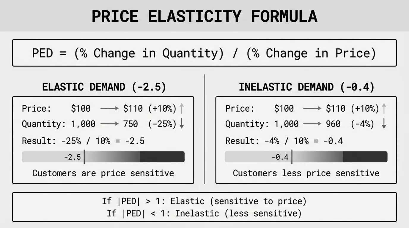
The price elasticity formula calculates how much quantity demanded changes when you change price. It's the ratio of percentage change in quantity to percentage change in price, expressed as PED = (% ΔQ) / (% ΔP). A coefficient of -1.5 means a 10% price increase causes a 15% drop in quantity demanded.

Price Elasticity Formula

The formula itself is straightforward. The hard part is interpreting what the number tells you about how to price, and understanding when B2B markets behave differently than the textbook examples.

The Basic Price Elasticity Formula

Price elasticity of demand is calculated by dividing the percentage change in quantity demanded by the percentage change in price.

PED = (% Change in Quantity Demanded) / (% Change in Price)
Or expressed with variables:
PED = ((Q₂ - Q₁) / Q₁) / ((P₂ - P₁) / P₁)
Where:
Q₁ = Original quantity demanded
Q₂ = New quantity demanded
P₁ = Original price
P₂ = New price

The result is almost always negative because price and quantity move in opposite directions. When price goes up, quantity goes down. When price goes down, quantity goes up. That's the law of demand.

Most economists report the absolute value (dropping the negative sign) to simplify interpretation. A coefficient of 2.0 is "more elastic" than 0.5, without having to remember that -2.0 is algebraically less than -0.5.

Worked Example: Basic Formula

An electrical distributor sells a common breaker panel at $180. They sell 400 units per month. They increase the price to $210. Sales drop to 320 units per month. What's the price elasticity?

Step 1: Calculate percentage change in quantity

(Q₂ - Q₁) / Q₁ = (320 - 400) / 400 = -80 / 400 = -0.20 = -20%

Step 2: Calculate percentage change in price

(P₂ - P₁) / P₁ = (210 - 180) / 180 = 30 / 180 = 0.167 = 16.7%

Step 3: Divide quantity change by price change

PED = -20% / 16.7% = -1.20

The price elasticity coefficient is -1.20 (or 1.20 in absolute value). This product is elastic. A 1% price increase causes a 1.2% decrease in quantity demanded. The distributor lost more volume than they gained in per-unit margin.

Revenue impact: Original revenue was $72,000/month (400 x $180). New revenue is $67,200/month (320 x $210). They raised price and lost $4,800/month in revenue. That's what elastic demand looks like in practice.

The Midpoint Method (Arc Elasticity Formula)

The basic formula has a problem. It gives different results depending on which direction you move.

Say you increase price from $100 to $120, and quantity drops from 200 to 150 units. Then you reverse the decision and drop price back to $100, and quantity returns to 200. Using the basic formula:

Price increase: 20% price change, -25% quantity change = elasticity of -1.25
Price decrease: -16.7% price change, 33.3% quantity change = elasticity of -2.0

Same product. Same price points. Different elasticity coefficients. That's a measurement problem, not a real economic change.

The midpoint method fixes this by using the average of the starting and ending values instead of just the starting value. It's also called arc elasticity because it measures elasticity over an arc (range) rather than at a point.

PED = ((Q₂ - Q₁) / ((Q₁ + Q₂) / 2)) / ((P₂ - P₁) / ((P₁ + P₂) / 2))
Simplified:
PED = ((Q₂ - Q₁) / (Q₁ + Q₂)) / ((P₂ - P₁) / (P₁ + P₂))

This looks more complex, but the logic is simple. Instead of dividing the change by the starting value, you divide by the average of starting and ending values. The midpoint method produces the same elasticity coefficient whether you're measuring a price increase or a price decrease between the same two points.

Worked Example: Midpoint Method

A fastener distributor sells stainless steel bolts at $2.50 per box with demand of 5,000 boxes per quarter. They test a price of $3.00 per box. Demand drops to 4,000 boxes. What's the price elasticity using the midpoint method?

Step 1: Calculate the average quantity

Average Q = (Q₁ + Q₂) / 2 = (5,000 + 4,000) / 2 = 4,500

Step 2: Calculate the average price

Average P = (P₁ + P₂) / 2 = (2.50 + 3.00) / 2 = 2.75

Step 3: Calculate percentage change in quantity using the average

% Change Q = (Q₂ - Q₁) / Average Q = (4,000 - 5,000) / 4,500 = -1,000 / 4,500 = -0.222 = -22.2%

Step 4: Calculate percentage change in price using the average

% Change P = (P₂ - P₁) / Average P = (3.00 - 2.50) / 2.75 = 0.50 / 2.75 = 0.182 = 18.2%

Step 5: Divide

PED = -22.2% / 18.2% = -1.22

The price elasticity is -1.22 using the midpoint method. If you reverse the calculation (starting from $3.00 and dropping to $2.50), you get the same coefficient. That's the advantage.

Revenue check: Original revenue was $12,500/quarter (5,000 x $2.50). New revenue is $12,000/quarter (4,000 x $3.00). Revenue decreased slightly. The product is just elastic enough that the price increase didn't improve total revenue.

Interpreting the Results: Elastic vs Inelastic

The coefficient tells you how sensitive customers are to price changes. Here's how to read it:

Coefficient	Interpretation	What It Means for Pricing
0 to -1	Inelastic	Customers aren't very price sensitive. Price increases don't lose much volume. Revenue goes up when you raise price.
Exactly -1	Unit elastic	Price and quantity changes offset perfectly. Revenue stays constant whether you raise or lower price.
Less than -1 (e.g., -2.5)	Elastic	Customers are price sensitive. Price increases lose too much volume. Revenue goes down when you raise price.

The more negative the number, the more elastic the demand. A coefficient of -3.0 is more elastic than -1.5. That product loses volume faster when you raise price.

Examples by category:

Essential MRO supplies (bearings, fasteners, common electrical): Often elastic (-1.5 to -3.0). Customers know the market price and shop around. Small price differences drive large volume shifts.
Specialty or technical products: Often inelastic (-0.3 to -0.8). Customers value specific features, certifications, or compatibility. Price matters less than fit and availability.
Mission-critical OEM components: Highly inelastic (-0.1 to -0.4). Switching suppliers requires re-engineering. Price changes have minimal impact on short-term demand.

Price Elasticity in B2B: Why It's Different

Most price elasticity examples use consumer goods. Gas prices, coffee, movie tickets. B2B markets behave differently.

1. Demand lags price changes. In consumer markets, you raise the price of bananas and see the effect within days. In B2B, customers often have existing contracts, inventory buffers, and purchasing cycles. A price increase in February might not affect order patterns until the next quarterly review in April. You need longer observation windows.

2. Elasticity varies by customer segment, not just product. The same bearing might be elastic for one customer (a price-sensitive job shop with substitutes available) and inelastic for another (an OEM who has that bearing spec'd into 50,000 units of production). Segment-level elasticity matters more than product-level averages.

3. Relationships and switching costs matter more. Customers don't just compare price. They compare total cost of doing business — payment terms, delivery reliability, technical support, order minimums. A 5% price increase might be offset by better service that saves the customer 8% in operational costs. Traditional elasticity formulas don't capture this.

4. You need transaction data, not survey data. Consumer studies often use surveys ("How much would you buy if the price increased 10%?"). B2B buyers don't answer reliably. According to research from Zilliant, transaction data such as customer, product, and order data can be used to segment customers into small groups that have similar price response and measure the price elasticity on an ongoing basis for each segment.

Want to analyze margins across your entire catalog?

Pryse finds hidden margin leakage in 24 hours. One-time $1,499 diagnostic.

Try Pryse

When to Use Each Formula

Use the basic formula when:

You're forecasting the impact of a future price change
You're working with small price adjustments (under 5%)
You need a quick directional answer

Use the midpoint method when:

You're analyzing historical data to measure what happened
You're comparing elasticity across different products or segments
You need precision for larger price changes (10%+ movements)
You're presenting analysis to finance or executives who will scrutinize methodology

The midpoint method is considered more accurate for analysis. The basic formula is faster for estimation. In practice, if you're only making small adjustments (2-3% price increases), the formulas give similar results. The gap widens when price changes are large.

Common Mistakes When Calculating Price Elasticity

Mistake 1: Confusing correlation with causation. Price went up 5%. Volume went down 8%. You calculate elasticity of -1.6. But maybe volume dropped because a competitor launched a better product, or your lead times increased, or the customer's production slowed. Isolating the price effect from other factors is hard without controlled conditions.

Mistake 2: Using list price instead of pocket price. If your list price is $100 but your average pocket price (after discounts and rebates) is $78, and you raise the list price to $110 but pocket price only moves to $81, you didn't actually increase price by 10%. You increased it by 3.8%. Measure elasticity based on the price the customer actually pays.

Mistake 3: Calculating elasticity with insufficient data. You need multiple price-quantity observations to calculate meaningful elasticity. Two data points can produce a coefficient, but it might not be reliable. Ideally you want 12-24 months of transaction data across a range of prices.

Mistake 4: Ignoring segment differences. An average elasticity coefficient across all customers hides valuable information. Large national accounts might have elasticity of -2.5. Small local customers might have elasticity of -0.8. Averaging them gives -1.65, which is the wrong number to use for either segment.

Mistake 5: Treating elasticity as constant. Elasticity changes over time. During an economic boom, demand becomes less elastic (customers care less about price). During a downturn, it becomes more elastic (every dollar matters). Your 2022 elasticity data might not apply in 2026.

Calculating Elasticity in Excel or Your Pricing Tool

Most mid-market companies don't have dedicated pricing software. You can calculate elasticity in Excel if you have transaction data.

What you need:

Sales history with at least 12 months of data
Columns for: Date, Customer, Product, Quantity Sold, Price per Unit
Enough price variation to measure (if you never change price, you can't measure elasticity)

Steps:

Segment your data by product and customer type
Group by month or quarter
Calculate average price and total quantity for each period
Apply the midpoint formula between consecutive periods
Average the elasticity coefficients to get a segment-level estimate

This won't be as precise as dedicated software, but it's enough to identify which product categories are elastic vs inelastic and make better pricing decisions.

For a more sophisticated approach, pricing optimization tools like Zilliant and Vendavo use regression models to isolate price effects from other variables. But you don't need $100K software to start measuring elasticity. You just need transaction data and the formulas above.

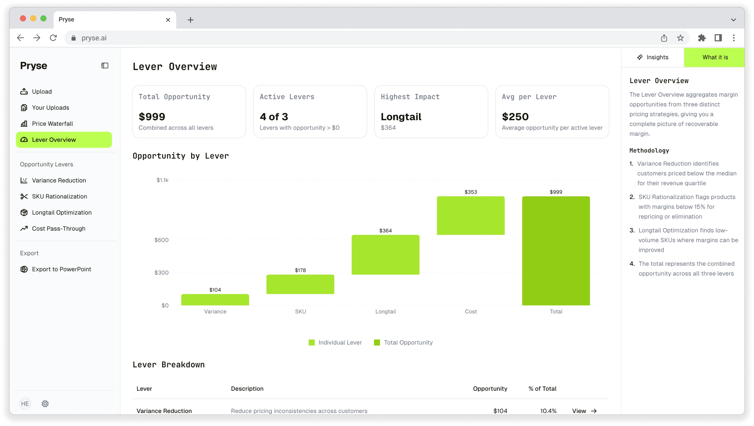
For companies that aren't ready for enterprise pricing software, a transaction analysis can reveal elasticity patterns. That's what Pryse's margin diagnostic does — it analyzes your pricing and margin data to show where you're leaving money on the table. You upload your data, and the tool identifies pricing inconsistencies and margin leakage that signal elasticity mismatches.

When Not to Trust the Formula

Price elasticity formulas assume rational, consistent behavior. B2B markets sometimes break those assumptions.

Contract pricing: If 60% of your volume is locked into 12-month contracts, elasticity calculations on list price are meaningless. The market can't respond to price changes until contracts renew.

Supply constraints: If you're capacity-limited or a product is on allocation, demand doesn't respond normally to price. You could raise price 20% and volume stays flat because you're sold out anyway.

Bundled pricing: If customers buy products in bundles or minimum order quantities, elasticity on individual SKUs is distorted. A 10% price increase on Product A might not reduce demand for Product A if customers need to hit a $5,000 minimum order anyway.

Switching costs vary by customer: Large customers with integrated systems have high switching costs (low elasticity). Small customers with no integration have low switching costs (high elasticity). A single elasticity coefficient can't represent both.

What to Do With Your Elasticity Coefficient

Calculating elasticity is useful. Acting on it is where the value is.

If demand is inelastic (coefficient between 0 and -1):

You can raise prices without losing significant volume
Revenue will increase when you raise price
Focus on margin expansion, not volume protection
Test 3-5% price increases on a segment and measure response

If demand is elastic (coefficient less than -1):

Price increases will cost you more volume than they're worth
Revenue will decrease if you raise price
Defend volume, don't chase margin
Look for cost reductions or differentiation that justifies price

If demand is unit elastic (coefficient near -1):

Price changes don't affect total revenue much
Focus on costs and operational efficiency instead
Small price increases are neutral to revenue but improve margin if costs stay flat

Next Steps

The formulas above work for any product where you have price and quantity data. The interpretation requires judgment. You're not just running the math — you're understanding your customers, your competitive position, and how price fits into your value proposition.

For more on how to use elasticity in your overall pricing strategy, see our complete Price Elasticity Guide.

If you want to see where pricing inconsistencies are hurting your margins across thousands of SKUs, start with a transaction data analysis. Pryse analyzes your pricing data to identify margin leakage and pricing opportunities — no elasticity calculations required.

Sources

Last updated: February 24, 2026