Price Elasticity: Complete Guide to Measuring Price Sensitivity
Learn price elasticity of demand: formulas, types, calculation methods, and B2B applications. Comprehensive guide with examples and real-world data.
Price elasticity of demand measures how quantity demanded changes when you change price. It's the ratio of percentage change in quantity to percentage change in price, calculated as PED = (% ΔQ) / (% ΔP). A coefficient of -1.5 means a 1% price increase causes a 1.5% decrease in quantity demanded.
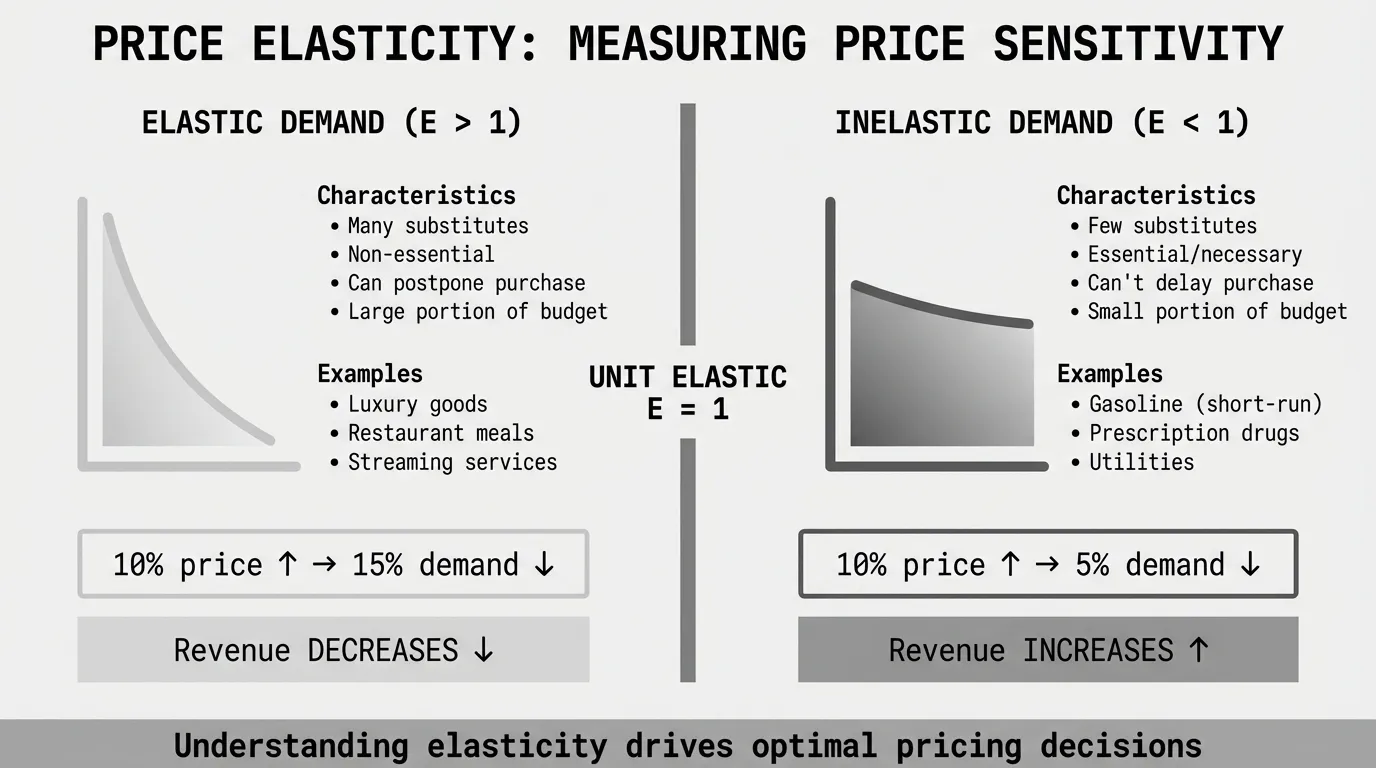
Understanding elasticity tells you whether raising price increases or decreases revenue. For elastic products (elasticity > 1), price increases reduce revenue because you lose too many customers. For inelastic products (elasticity < 1), price increases raise revenue because volume drops only slightly.
This guide covers the five types of elasticity, how to calculate and interpret the coefficient, what makes products elastic vs inelastic, and how B2B markets differ from consumer markets in measuring price sensitivity.
What Is Price Elasticity of Demand?
Price elasticity of demand is the percentage change in quantity demanded divided by the percentage change in price. It measures customer price sensitivity.
Price Elasticity of Demand = (% Change in Quantity Demanded) / (% Change in Price)
The result is almost always negative because price and quantity move in opposite directions. When price increases, quantity demanded decreases. When price decreases, quantity demanded increases. Most economists report the absolute value to simplify interpretation.
A coefficient of -2.0 is more elastic than -0.5, but comparing absolute values (2.0 vs 0.5) is easier than remembering that -2.0 is algebraically less than -0.5.
According to MasterClass's pricing guide, price elasticity of demand is one of the most important concepts in microeconomics and an essential metric for developing a company's pricing strategy.
Why Price Elasticity Matters
Knowing whether demand is elastic or inelastic determines optimal pricing strategy.
For elastic demand (coefficient > 1):
- Price increases reduce total revenue
- Price decreases increase total revenue
- Compete on price and volume
- Use discounts and promotions to drive sales
For inelastic demand (coefficient < 1):
- Price increases raise total revenue
- Price decreases reduce total revenue
- Compete on value, not price
- Focus on margin expansion through price increases
According to McKinsey research cited in C-Suite Strategy, a 1% improvement in pricing can lead to an 8.7% increase in operating profits—making pricing optimization far more impactful than comparable improvements in costs or volume.
Misunderstanding elasticity destroys value. Raising prices on elastic products drives customers away. Leaving prices low on inelastic products leaves money on the table.
The Five Types of Price Elasticity
Price elasticity falls into five categories based on the coefficient value.
| Type | Coefficient Range | Description | Revenue Effect |
|---|---|---|---|
| Perfectly Elastic | Infinity (∞) | Any price increase drops demand to zero | Can't raise price at all |
| Elastic | |E| > 1 | Demand changes more than price | Price ↑ = Revenue ↓ |
| Unit Elastic | |E| = 1 | Demand changes equal to price | Price ↑ = No revenue change |
| Inelastic | |E| < 1 | Demand changes less than price | Price ↑ = Revenue ↑ |
| Perfectly Inelastic | 0 | Demand doesn't change at all | Price ↑ = Revenue ↑ proportionally |
Perfectly Elastic Demand
Perfectly elastic demand means any price increase causes demand to drop to zero. The elasticity coefficient is infinite.
This happens in perfectly competitive markets where products are identical. If Farmer A sells wheat for $7.01 per bushel and Farmer B sells the same wheat for $7.00, everyone buys from Farmer B. Farmer A's demand drops to zero.
In practice, few products are truly perfectly elastic because of switching costs, convenience, or slight differentiation.
Elastic Demand
Elastic demand means the coefficient is greater than 1 in absolute value. A 10% price increase causes more than a 10% drop in quantity demanded.
Products with elastic demand typically have:
- Many substitutes (streaming services, fast food)
- Non-essential uses (luxury goods, entertainment)
- Purchases that can be postponed (furniture, vacations)
- High price visibility (commodities with published pricing)
Example: A streaming service raises its monthly price from $10 to $11 (10% increase). Subscriptions drop from 1 million to 850,000 (15% decrease). The elasticity coefficient is -1.5, indicating elastic demand.
When demand is elastic, lowering price increases revenue. The volume gain exceeds the price reduction.
For more elastic demand cases, see our post on price elasticity examples.
Unit Elastic Demand
Unit elastic demand means the coefficient equals exactly 1.0. A 10% price increase causes exactly a 10% drop in quantity demanded.
Revenue stays constant whether you raise or lower price. A 10% price increase combined with a 10% volume drop leaves total revenue unchanged.
Unit elasticity is rare in practice but represents the boundary between elastic and inelastic zones.
Inelastic Demand
Inelastic demand means the coefficient is less than 1 in absolute value. A 10% price increase causes less than a 10% drop in quantity demanded.
Products with inelastic demand typically have:
- Few substitutes (prescription drugs, electricity)
- Essential uses (gasoline in the short run, food staples)
- Purchases that can't be postponed (emergency repairs, medical care)
- Small portion of customer budget (salt, matches)
Example: An electrical distributor raises the price of safety switches from $50 to $55 (10% increase). Sales drop from 1,000 units to 950 units per month (5% decrease). The elasticity coefficient is -0.5, indicating inelastic demand.
When demand is inelastic, raising price increases revenue. The volume loss is smaller than the price gain.
Perfectly Inelastic Demand
Perfectly inelastic demand means quantity demanded stays exactly the same regardless of price changes. The elasticity coefficient is zero.
Insulin for Type 1 diabetics is the classic example. A patient who needs 30 units per day will buy 30 units whether it costs $10 or $100 per vial. There's no substitute and the quantity required is medically determined.
Few products are truly perfectly inelastic. Even insulin shows some elasticity as patients delay refills or ration doses when prices spike sharply.
How to Calculate Price Elasticity
There are two methods for calculating price elasticity: the basic formula and the midpoint method.
Basic Formula
The basic formula calculates percentage changes from the starting values.
PED = ((Q₂ - Q₁) / Q₁) / ((P₂ - P₁) / P₁)
Where:
Q₁ = Original quantity demanded
Q₂ = New quantity demanded
P₁ = Original price
P₂ = New price
Worked Example:
An HVAC distributor sells a motor at $200. They sell 500 units per month. They raise the price to $240. Sales drop to 420 units per month.
Step 1: Calculate percentage change in quantity.
(420 - 500) / 500 = -80 / 500 = -0.16 = -16%
Step 2: Calculate percentage change in price.
(240 - 200) / 200 = 40 / 200 = 0.20 = 20%
Step 3: Divide quantity change by price change.
PED = -16% / 20% = -0.8
The coefficient is -0.8, meaning demand is inelastic. The 20% price increase caused only a 16% drop in volume, so total revenue increased from $100,000 to $100,800 per month.
Midpoint Formula
The midpoint method uses the average of starting and ending values instead of just the starting values. This gives the same result whether price increases or decreases.
PED = [(Q₂ - Q₁) / ((Q₂ + Q₁) / 2)] / [(P₂ - P₁) / ((P₂ + P₁) / 2)]
According to Lumen Learning's microeconomics course, the midpoint method for elasticity uses the average percentage change in both quantity and price, providing consistent results regardless of direction.
Why use the midpoint method? The basic formula gives different results depending on whether price is increasing or decreasing. If price goes from $10 to $12, then back to $10, you get two different elasticity coefficients. The midpoint method eliminates this asymmetry.
When to use each method:
- Basic formula: Quick estimates, comparing elasticity across products
- Midpoint formula: Analyzing historical price changes, academic research, reporting consistent metrics
For step-by-step calculation guidance with B2B examples, see our post on price elasticity formula.
Interpreting the Price Elasticity Coefficient
The elasticity coefficient tells you three things: sensitivity level, revenue impact, and optimal strategy.
Reading the Coefficient Value
According to ReviewEcon's elasticity guide, here's how to interpret common coefficient ranges:
| Coefficient | Interpretation | Price Increase Impact |
|---|---|---|
| -3.0 to -2.0 | Highly elastic | 10% price increase → 20-30% volume drop |
| -2.0 to -1.0 | Elastic | 10% price increase → 10-20% volume drop |
| -1.0 | Unit elastic | 10% price increase → 10% volume drop |
| -0.5 to -1.0 | Slightly inelastic | 10% price increase → 5-10% volume drop |
| -0.5 to -0.2 | Inelastic | 10% price increase → 2-5% volume drop |
| -0.2 to 0 | Highly inelastic | 10% price increase → 0-2% volume drop |
Revenue Impact
Revenue equals price times quantity. Elasticity determines which effect dominates.
Elastic demand (coefficient > 1):
Raising price from $100 to $110 (10% increase) drops quantity from 1,000 to 800 units (20% decrease, coefficient = -2.0).
Old Revenue = $100 × 1,000 = $100,000
New Revenue = $110 × 800 = $88,000
Revenue Change = -$12,000 (-12%)
The volume loss exceeds the price gain. Revenue falls.
Inelastic demand (coefficient < 1):
Raising price from $100 to $110 (10% increase) drops quantity from 1,000 to 950 units (5% decrease, coefficient = -0.5).
Old Revenue = $100 × 1,000 = $100,000
New Revenue = $110 × 950 = $104,500
Revenue Change = +$4,500 (+4.5%)
The price gain exceeds the volume loss. Revenue increases.
What Makes Demand Elastic vs Inelastic?
Four factors determine whether demand is elastic or inelastic: availability of substitutes, necessity level, time horizon, and budget proportion.
Availability of Substitutes
Products with many substitutes have elastic demand. Customers switch when price increases.
Elastic examples:
- Commodity fasteners—customers can buy from dozens of distributors
- Generic office supplies—abundant alternatives at similar quality
- Streaming services—Netflix, Disney+, Hulu, Max, Apple TV+ compete directly
Inelastic examples:
- Mission-critical OEM components with single-source suppliers
- Proprietary software with high switching costs
- Patented pharmaceuticals with no generic alternatives
According to Zilliant's B2B elasticity analysis, in B2B manufacturing, a company may be the exclusive supplier of a particular component, and demand is more likely to correlate with the demand for the end product rather than its own price.
Necessity Level
Essential products have inelastic demand. Customers need them regardless of price.
Inelastic examples:
- Industrial safety equipment required by regulation
- Critical spare parts for production equipment
- Utilities (electricity, water, gas)
Elastic examples:
- Luxury office furniture upgrades
- Premium packaging materials when standard options exist
- Discretionary consulting services
Time Horizon
Demand becomes more elastic over time as customers adjust behavior and find alternatives.
Gasoline example:
- Short run (weeks): Highly inelastic (coefficient around -0.2). People need to drive to work.
- Medium run (months): Slightly inelastic (coefficient around -0.5). People carpool or use public transit.
- Long run (years): Elastic (coefficient around -1.5). People buy fuel-efficient cars or move closer to work.
Budget Proportion
Products that consume a small portion of the customer's budget tend to be inelastic. The price change isn't material enough to alter behavior.
Inelastic examples:
- Salt, matches, paper clips—price changes are measured in pennies
- Small fasteners or consumables in a multi-million dollar factory
- Low-cost MRO items ordered automatically
Elastic examples:
- Capital equipment purchases consuming months of budget
- Large raw material contracts affecting total product cost
- Major software licenses representing significant IT spend
Price Elasticity in B2B Markets
B2B price elasticity differs from consumer markets in three ways: it varies more by customer segment, relationship strength matters, and demand is often derived from end-customer demand.
Segment Variation
B2B elasticity varies dramatically by customer type, purchase context, and competitive situation.
According to PricingBrew's B2B elasticity analysis, B2B customers buy out of necessity, not impulse. If you need two motors, you buy two motors. A steep discount might lead you to buy three, but that just means you'll postpone buying the third one you would have bought later.
High elasticity segments:
- Commodity products with published market pricing
- Spot buyers with no relationship or contract
- Large customers who can negotiate or switch easily
- Price-sensitive industries with thin margins
Low elasticity segments:
- Mission-critical components for production
- Long-term contract customers with switching costs
- Small customers where switching effort exceeds savings
- Highly specified products with few qualified alternatives
Derived Demand
B2B demand is often derived from end-customer demand, not the component price itself.
An automotive parts manufacturer sells brake assemblies to car makers. If car sales are strong, the manufacturer needs brake assemblies regardless of whether the price is $50 or $55 per unit. Demand tracks vehicle production, not brake prices.
According to B2B Frameworks' elasticity overview, in industrial applications, demand cannot increase because the need is determined by the volume output of whatever the components are used in.
This makes B2B demand appear inelastic in the short run. Over time, if brake prices increase 20%, car manufacturers might redesign for cheaper alternatives or switch suppliers, but that takes months or years.
Relationship vs Transactional
Long-term B2B relationships reduce price elasticity. Switching costs include requalifying suppliers, testing new products, training staff, and integration effort.
A distributor who's been supplying a manufacturer for 10 years has lower elasticity than a spot supplier. The relationship creates friction that dampens price sensitivity.
Conversely, purely transactional B2B markets (commodity chemicals, generic fasteners, standard components) show high elasticity similar to consumer markets.
Cross-Price Elasticity
Cross-price elasticity measures how demand for Product A changes when the price of Product B changes.
Cross-Price Elasticity = (% Change in Quantity of A) / (% Change in Price of B)
Positive cross-elasticity: Products are substitutes. Raising the price of Coke increases Pepsi demand.
Negative cross-elasticity: Products are complements. Raising printer prices reduces ink demand.
Near-zero cross-elasticity: Products are unrelated. Raising bread prices doesn't affect tire sales.
B2B Applications
Cross-price elasticity helps with:
- Pricing product families: If raising price on Product A drives customers to cheaper Product B in your catalog, you capture revenue either way
- Competitive response: Understanding which competitor's products are true substitutes
- Bundle pricing: Identifying complementary products to package together
A distributor might discover that raising prices on premium bearings increases demand for standard bearings by 8%. The cross-price elasticity is positive, confirming they're substitutes. Some customers downgrade when the premium option gets too expensive.
For detailed cross-price analysis, see our post on cross-price elasticity.
Income Elasticity of Demand
Income elasticity measures how demand changes when customer income changes. It's separate from price elasticity but follows similar logic.
Income Elasticity = (% Change in Quantity Demanded) / (% Change in Income)
Normal goods (positive income elasticity): Demand increases when income rises. Most products fall here.
Luxury goods (income elasticity > 1): Demand increases faster than income. International travel, premium brands.
Inferior goods (negative income elasticity): Demand decreases when income rises. Instant ramen, public transit, generic store brands. Customers upgrade to better alternatives when they can afford it.
For B2B markets, income elasticity relates to industry health. When manufacturers are profitable, they upgrade to premium supplies and faster delivery. During downturns, they switch to cheaper alternatives.
For more detail, see our guide on income elasticity of demand.
Using Price Elasticity for Pricing Decisions
Once you know elasticity, you can set optimal prices by segment, product, and customer.
Segmented Pricing
Price by elasticity to maximize revenue across customer segments.
Strategy for elastic segments:
- Compete on price and value
- Offer volume discounts and promotions
- Focus on convenience and service differentiation
- Avoid price increases unless necessary
Strategy for inelastic segments:
- Charge higher prices to capture margin
- Focus on availability, reliability, speed
- Resist discounting pressure
- Regularly increase prices to match value
Airlines use this when charging business travelers (inelastic) 3x what leisure travelers (elastic) pay for the same seat. Both segments fill the plane, but at different price points.
Product Portfolio Management
Segment your product catalog by elasticity to optimize pricing across SKUs.
High elasticity products:
- Match or undercut competitive pricing
- Use as traffic drivers or loss leaders
- Focus on operational efficiency to maintain margin
- Consider exiting if margins stay weak
Low elasticity products:
- Price for margin, not market share
- Implement regular price increases
- Invest in product differentiation
- Protect through patents, specifications, or relationships
A distributor analyzed 50,000 SKUs and found 12% had inelastic demand (elasticity < 0.5) but generated 40% of gross margin dollars. They increased prices 8-15% on those SKUs over 18 months with minimal volume loss, adding $1.8 million in annual gross profit.
Dynamic Pricing
Monitor elasticity over time to adjust prices as market conditions change.
Elasticity isn't static. Products become more elastic as:
- Substitutes emerge (competitors launch comparable products)
- Customer knowledge increases (price transparency through online marketplaces)
- Switching costs decline (standardization makes suppliers interchangeable)
- Economic conditions weaken (customers become more price-sensitive)
Companies using advanced analytics in pricing achieve 2-7% higher margins than competitors who don't, according to McKinsey research.
Measure elasticity quarterly for high-volume products. Annual reviews work for slower-moving items. Adjust pricing strategy when elasticity shifts meaningfully (more than 0.3 change in coefficient).
Measuring Price Elasticity: Data Requirements
Calculating elasticity requires transaction data across different price points and time periods.
Minimum Data Requirements
To measure elasticity, you need:
- At least 50-100 transactions per product or segment
- Price variation of 10% or more across the dataset
- Time series data (6-12 months minimum) or cross-sectional data (multiple price points simultaneously)
- Quantity demanded at each price point
Challenges:
- Many B2B companies don't have enough price variation to calculate elasticity reliably
- Contract pricing stays fixed for 12 months, eliminating variation
- Product mix changes confound the analysis (are sales declining because of price or because customers switched products?)
Sources of Price Variation
If you don't have natural price variation, these situations provide data:
Historical price changes: Analyze how volume responded when you raised or lowered prices in the past.
Geographic pricing: Different regions often have different prices. Compare demand across regions.
Customer segments: You charge different prices to different customer types. Compare volume across segments.
Competitive pricing: Track what happens when competitors change prices. Your volume responds to their elasticity.
Promotional periods: Compare normal-price demand to discounted-demand during promotions.
Regression Analysis
For products with sufficient data, regression analysis estimates elasticity more accurately than simple before/after comparisons.
The regression model predicts quantity demanded based on price, controlling for other factors like seasonality, marketing spend, competitor pricing, and economic conditions.
A typical regression might find that each $1 increase in price reduces monthly quantity by 12 units on average. Combined with average price and quantity, this translates to an elasticity coefficient.
This is beyond what most mid-market companies do in Excel. Specialized pricing analytics software automates the regression and reports elasticity by product and customer segment.
Common Mistakes in Elasticity Analysis
Five mistakes distort elasticity calculations and lead to wrong pricing decisions.
Ignoring Non-Price Factors
Volume changes aren't always caused by price changes. Demand shifts because of:
- Seasonality (HVAC demand peaks in summer)
- Economic conditions (recessions reduce industrial purchasing)
- Competitor actions (a competitor exit drives volume to you)
- Marketing activity (a promotion increases awareness independent of price)
- Product quality changes (an improved version sells more at the same price)
Don't attribute all volume changes to price. Control for other variables or use regression analysis.
Using Too Short a Time Period
Elasticity measured over one month is noisier than elasticity measured over a year. Short-term fluctuations (inventory destocking, budget freezes, one-time projects) distort the signal.
Use at least 6 months of data. A year is better. Multiple years helps if the product and market haven't changed significantly.
Averaging Across Heterogeneous Segments
Calculating one elasticity coefficient across all customers hides critical variation.
A distributor found overall elasticity of -0.8 for a product line. When segmented:
- Large national accounts: -1.5 (elastic, price-sensitive)
- Regional mid-market: -0.6 (inelastic, relationship-based)
- Small local customers: -0.3 (highly inelastic, convenience-focused)
Pricing the product uniformly based on -0.8 leaves money on the table with small customers and loses share with large customers.
Always segment by customer size, industry, purchase frequency, or relationship type before calculating elasticity.
Confusing Movement Along vs Shift of Demand Curve
Movement along the demand curve: You change price, quantity demanded responds. This is elasticity.
Shift of the demand curve: External factors change demand at every price level. The entire relationship shifts.
If a new regulation requires safety equipment, demand increases at all price levels. That's a demand shift, not elasticity. Raising price during a demand surge doesn't reveal elasticity—it just captures increased willingness to pay.
Treating Elasticity as Constant
Elasticity changes based on price level. A product might be inelastic from $50 to $60 but elastic from $100 to $110.
As price increases, more substitutes become economically viable. At $50, the motor has no good substitutes. At $100, three competitors' products become cheaper alternatives. Elasticity increases.
Calculate elasticity within relevant price ranges. Don't extrapolate coefficients far beyond the data used to estimate them.
Industry Benchmarks and Typical Elasticity Ranges
Elasticity varies by industry, product type, and market structure. General ranges:
| Industry/Product Category | Typical Elasticity Range |
|---|---|
| Consumer Goods | |
| Eggs | -0.1 to -0.3 (highly inelastic) |
| Milk | -0.3 to -0.6 (inelastic) |
| Gasoline (short run) | -0.2 to -0.3 (inelastic) |
| Gasoline (long run) | -1.2 to -1.8 (elastic) |
| Restaurant meals | -1.6 to -2.3 (elastic) |
| Airline tickets (leisure) | -1.5 to -2.5 (elastic) |
| Luxury cars | -2.0 to -3.0 (highly elastic) |
| B2B Industrial | |
| Mission-critical OEM components | -0.1 to -0.4 (highly inelastic) |
| Commodity MRO supplies | -1.5 to -2.5 (elastic) |
| Specialty chemicals | -0.4 to -0.8 (inelastic) |
| Standard electrical components | -1.0 to -1.8 (elastic) |
| Custom fabricated parts | -0.3 to -0.6 (inelastic) |
| Services | |
| Healthcare (insured) | -0.2 to -0.4 (inelastic) |
| Business consulting | -1.0 to -1.5 (elastic) |
| Software subscriptions | -1.5 to -2.5 (elastic) |
These are directional ranges, not precise measurements. Your actual elasticity depends on competitive position, customer relationships, and specific market dynamics.
Tools for Calculating Price Elasticity
Most mid-market companies start with Excel before investing in specialized software.
Excel Analysis
You can calculate elasticity in Excel with transaction data exported from your ERP:
- Export sales history with date, product, quantity, price, customer
- Calculate percentage change in quantity and price period-over-period
- Divide quantity change by price change for each product
- Average the coefficients across time periods or customer segments
This works for quick estimates on high-volume products. Limitations include difficulty controlling for non-price factors and handling thousands of SKUs.
Price Elasticity Calculators
Online calculators let you input before/after price and quantity to get an instant coefficient.
Our price elasticity calculator supports both the basic formula and midpoint method. You can also use the price elasticity of demand calculator for step-by-step guidance.
Calculators work for one-off analysis but don't scale to analyzing thousands of products systematically.
Pricing Analytics Software
Specialized pricing software automates elasticity calculation across products and customer segments using regression analysis.
These tools:
- Import transaction data from your ERP automatically
- Calculate elasticity by product, customer, region, channel
- Control for seasonality, competition, economic factors
- Recommend optimal prices by segment
- Simulate revenue impact of price changes
Enterprise solutions (PROS, Vendavo, Zilliant) cost $100K-$500K annually and target large companies with complex pricing. Mid-market alternatives include self-serve analytics tools starting under $10K annually.
For more on pricing software categories, see our guide on pricing optimization.
Price Elasticity and Margin Analysis
Price elasticity should inform pricing decisions alongside margin analysis. High elasticity doesn't mean low prices are optimal if your margins can't support volume growth.
Combining Elasticity and Margin Data
Calculate profit-maximizing price by considering both elasticity and margin structure.
Example: A product has:
- Current price: $100
- Current cost: $70
- Current margin: 30%
- Current volume: 1,000 units/month
- Price elasticity: -0.8 (inelastic)
Scenario 1: Raise price to $110
Volume drops to 920 units (8% decrease from 10% price increase).
Current Profit = ($100 - $70) × 1,000 = $30,000
New Profit = ($110 - $70) × 920 = $36,800
Profit Increase = +$6,800 (+23%)
Scenario 2: Lower price to $90
Volume increases to 1,080 units (8% increase from 10% price decrease).
Current Profit = ($100 - $70) × 1,000 = $30,000
New Profit = ($90 - $70) × 1,080 = $21,600
Profit Decrease = -$8,400 (-28%)
For inelastic products with healthy margins, price increases drive profit even when volume declines. The margin expansion exceeds volume loss.
For elastic products or low-margin products, the math changes. Volume becomes critical to covering fixed costs.
Margin Leakage and Elasticity
Companies often assume demand is more elastic than it actually is because they see price sensitivity in customer negotiations. But negotiated discounts don't reveal true elasticity—they reveal your willingness to discount.
According to McKinsey research cited in GetMonetizely's pricing guide, companies that regularly analyze pricing waterfalls identify 3-8% more margin opportunity than those who don't.
Many distributors could raise prices 5-10% on inelastic product segments without meaningful volume loss, but they don't because salespeople preemptively discount to "stay competitive."
Test elasticity with actual price increases, not salesperson intuition. You might discover demand is far more inelastic than assumed.
For more on identifying margin opportunities, see our guide on margin leakage.
Summary
Price elasticity of demand measures customer price sensitivity by calculating the ratio of percentage change in quantity to percentage change in price. Products with elastic demand (coefficient > 1) see revenue decline when prices increase because volume drops sharply. Products with inelastic demand (coefficient < 1) see revenue increase when prices rise because volume drops only slightly.
Understanding elasticity by product and customer segment lets you price for profit rather than market share alone. Elastic segments need competitive pricing and volume strategies. Inelastic segments can support price increases that expand margin.
B2B markets show different elasticity patterns than consumer markets. Demand is often derived from end-customer needs, not component pricing. Relationships and switching costs reduce price sensitivity. Segmentation matters more because elasticity varies dramatically by customer type and purchase context.
Measure elasticity using transaction data across different price points. Calculate coefficients by product and customer segment. Test pricing changes to validate assumptions. Use the insights to set prices that maximize profit, not just revenue.
For calculation guidance, see our post on price elasticity formula. For real-world examples across industries, see price elasticity examples. For specific elasticity types, explore cross-price elasticity and price elasticity of supply.
Sources:
- How to Calculate Price Elasticity of Demand - MasterClass
- Price Elasticity of Demand Formula - Wall Street Mojo
- Calculating Price Elasticities Using the Midpoint Formula - Lumen Learning
- The Strategic Edge of Pricing Power - C-Suite Strategy
- Price Elasticity in B2B - Zilliant
- Price Elasticity in B2B: Who's Right? - PricingBrew
- Price Elasticity - B2B Frameworks
- Elasticity Coefficients - ReviewEcon
Last updated: February 24, 2026
Related Articles
Frequently Asked Questions
Want to analyze your entire product catalog?
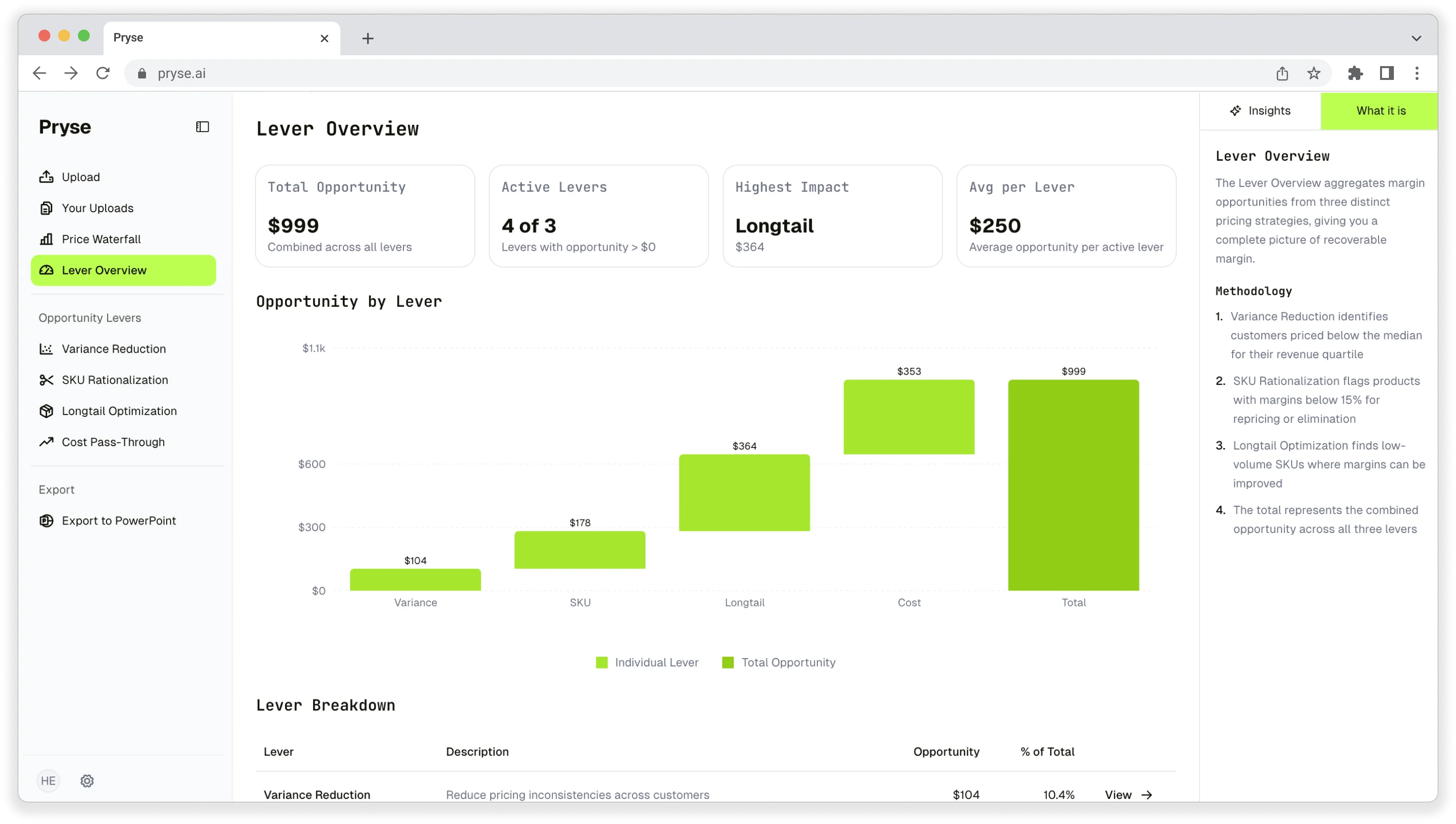
Pryse automatically identifies margin leakage across thousands of SKUs. Upload your data and find hidden profit in 24 hours.
One-time $1,499 diagnostic. No subscription required.