Price Elasticity of Demand Midpoint Formula: Consistent Calculations
The midpoint formula calculates price elasticity consistently regardless of direction. Learn when to use arc elasticity vs basic PED with B2B examples.
The price elasticity of demand midpoint formula calculates elasticity using the average of starting and ending values for both price and quantity. It's expressed as PED = ((Q₂ - Q₁) / ((Q₁ + Q₂) / 2)) / ((P₂ - P₁) / ((P₁ + P₂) / 2)). This method produces the same coefficient whether you're measuring a price increase or decrease.
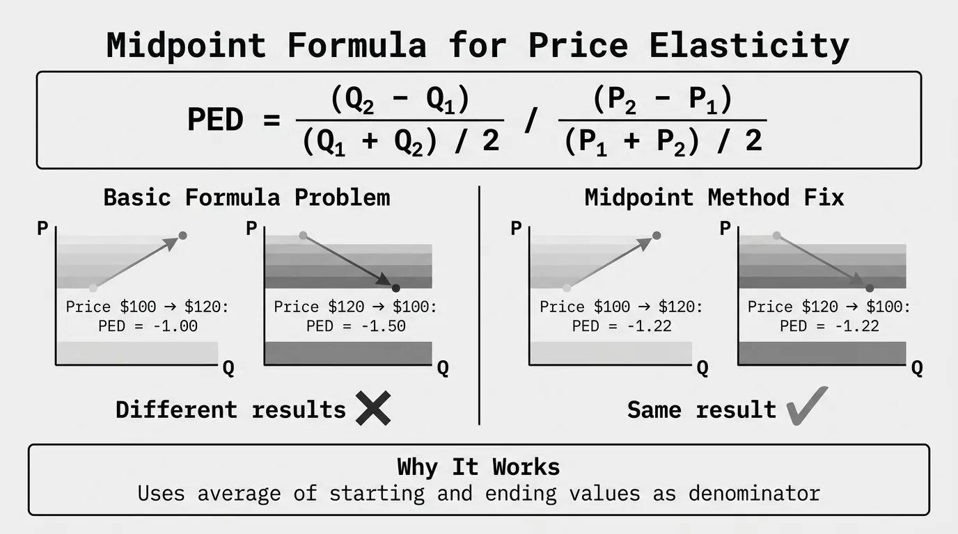
The midpoint formula solves the directional bias problem in the basic price elasticity calculation. If you raise price from $10 to $12, then drop it back to $10, the basic formula gives different elasticity coefficients for each change. The midpoint method gives the same coefficient both directions.
The Problem With the Basic Formula
The basic price elasticity formula calculates percentage changes using the starting value as the denominator. This creates a directional bias.
Here's why. Say you sell industrial valves at $100 each with demand of 500 units per month. You test a price increase to $120. Demand drops to 400 units.
Using the basic formula:
Percentage change in quantity:
(400 - 500) / 500 = -100 / 500 = -0.20 = -20%
Percentage change in price:
(120 - 100) / 100 = 20 / 100 = 0.20 = 20%
Price elasticity of demand:
PED = -20% / 20% = -1.00
Now reverse it. You drop the price back to $100 and demand returns to 500 units.
Going from $120 to $100:
Percentage change in quantity:
(500 - 400) / 400 = 100 / 400 = 0.25 = 25%
Percentage change in price:
(100 - 120) / 120 = -20 / 120 = -0.167 = -16.7%
Price elasticity of demand:
PED = 25% / -16.7% = -1.50
Same product. Same two price points. Different elasticity coefficients: -1.00 vs -1.50. That's a measurement problem, not a real economic difference.
The bias comes from using different denominators. Going up, you divide by the smaller starting values (500 units, $100). Going down, you divide by the larger starting values (400 units, $120). Different denominators produce different percentage changes even when the absolute changes are identical.
How the Midpoint Formula Fixes This
The midpoint method, also called arc elasticity, uses the average of the starting and ending values as the denominator for both calculations.
PED = ((Q₂ - Q₁) / ((Q₁ + Q₂) / 2)) / ((P₂ - P₁) / ((P₁ + P₂) / 2))
You can simplify this by multiplying the numerator and denominator:
PED = ((Q₂ - Q₁) / (Q₁ + Q₂)) / ((P₂ - P₁) / (P₁ + P₂))
Both formulas are mathematically equivalent. The second version is slightly faster to calculate because you don't need to divide by 2 twice.
According to Lumen Learning's microeconomics course, the advantage of the midpoint method is that one obtains the same elasticity between two price points whether there is a price increase or decrease.
Worked Example: Midpoint Method
Let's recalculate the valve example using the midpoint method.
From $100 to $120 (price increase):
Step 1: Calculate average quantity and price.
Average Q = (500 + 400) / 2 = 450
Average P = (100 + 120) / 2 = 110
Step 2: Calculate percentage changes using the averages.
% Change in Q = (400 - 500) / 450 = -100 / 450 = -0.222 = -22.2%
% Change in P = (120 - 100) / 110 = 20 / 110 = 0.182 = 18.2%
Step 3: Calculate elasticity.
PED = -22.2% / 18.2% = -1.22
From $120 to $100 (price decrease):
Step 1: Calculate average quantity and price.
Average Q = (400 + 500) / 2 = 450
Average P = (120 + 100) / 2 = 110
Step 2: Calculate percentage changes using the averages.
% Change in Q = (500 - 400) / 450 = 100 / 450 = 0.222 = 22.2%
% Change in P = (100 - 120) / 110 = -20 / 110 = -0.182 = -18.2%
Step 3: Calculate elasticity.
PED = 22.2% / -18.2% = -1.22
Both directions give -1.22. The midpoint method eliminates the directional bias.
Another Example: Building Materials Distributor
A distributor sells drywall at $12 per sheet with demand of 8,000 sheets per month. They raise the price to $13.50. Demand drops to 7,200 sheets. What's the price elasticity using the midpoint formula?
Step 1: Calculate averages
Average Q = (8,000 + 7,200) / 2 = 7,600
Average P = (12.00 + 13.50) / 2 = 12.75
Step 2: Calculate percentage changes
% Change in Q = (7,200 - 8,000) / 7,600 = -800 / 7,600 = -0.105 = -10.5%
% Change in P = (13.50 - 12.00) / 12.75 = 1.50 / 12.75 = 0.118 = 11.8%
Step 3: Calculate elasticity
PED = -10.5% / 11.8% = -0.89
The coefficient is -0.89. This product is inelastic. Customers are not very price sensitive. The distributor can raise prices without losing significant volume.
Revenue check: Original revenue was $96,000/month (8,000 × $12). New revenue is $97,200/month (7,200 × $13.50). Revenue increased by $1,200 despite losing 800 units. That's how inelastic demand works.
Midpoint Formula vs Basic Formula: When to Use Each
| Scenario | Best Method | Reason |
|---|---|---|
| Analyzing historical price changes | Midpoint | Gives consistent results for retrospective analysis |
| Forecasting impact of future price change | Basic | Simpler calculation, directional bias doesn't matter |
| Comparing elasticity across products | Midpoint | Eliminates bias when price changes vary by size |
| Small price adjustments (under 5%) | Either | Results are similar for small changes |
| Large price movements (over 10%) | Midpoint | Basic formula becomes increasingly biased |
| Presenting to executives or finance | Midpoint | More accurate and defensible methodology |
| Quick estimate for pricing decision | Basic | Faster, directional answer is good enough |
According to Pearson's microeconomics resources, the midpoint method is the standard approach taught in economics courses because it produces consistent results.
Step-by-Step Calculation Guide
Here's a template you can use for any midpoint elasticity calculation:
Step 1: Gather your data
- Q₁ = Quantity demanded at original price
- Q₂ = Quantity demanded at new price
- P₁ = Original price
- P₂ = New price
Step 2: Calculate averages
- Average Q = (Q₁ + Q₂) / 2
- Average P = (P₁ + P₂) / 2
Step 3: Calculate percentage changes
- % Change in Q = (Q₂ - Q₁) / Average Q × 100
- % Change in P = (P₂ - P₁) / Average P × 100
Step 4: Calculate elasticity
- PED = (% Change in Q) / (% Change in P)
Step 5: Interpret the result
- If PED is between 0 and -1: inelastic demand
- If PED is exactly -1: unit elastic demand
- If PED is less than -1 (like -2.5): elastic demand
Calculating Midpoint Elasticity in Excel
You can build a simple midpoint elasticity calculator in Excel:
Cell setup:
- A2: Q1 (original quantity)
- B2: Q2 (new quantity)
- C2: P1 (original price)
- D2: P2 (new price)
Formulas:
- E2: Average Q =
=(A2+B2)/2 - F2: Average P =
=(C2+D2)/2 - G2: % Change Q =
=(B2-A2)/E2 - H2: % Change P =
=(D2-C2)/F2 - I2: PED =
=G2/H2
Enter your data in rows 2 onward. The PED coefficient appears in column I.
This works for single calculations or batch analysis across hundreds of products if you have transaction data exported from your ERP.
Arc Elasticity vs Point Elasticity
The midpoint method calculates arc elasticity — elasticity measured over an arc (range) between two points. There's another method called point elasticity that measures elasticity at a specific point on the demand curve.
Arc elasticity:
- Uses two data points (before and after a price change)
- Practical for business applications
- Calculated with the midpoint formula
- Gives average elasticity over the range
Point elasticity:
- Uses calculus to measure elasticity at an exact point
- Requires knowing the demand function equation
- More precise but harder to calculate
- Used in academic economics
For B2B pricing decisions, arc elasticity is more useful. You have transaction data showing what happened before and after price changes. You rarely have a precise demand function.
According to Economics Online, the midpoint method remains the standard approach for business analysis because it only requires two observable data points.
Common Mistakes When Using the Midpoint Formula
Mistake 1: Forgetting to use averages for both price and quantity. Some people calculate average price but forget to calculate average quantity (or vice versa). Both must use the midpoint.
Mistake 2: Mixing up the order of Q₂ and Q₁. If you're measuring a price increase from $10 to $12, make sure Q₁ is the quantity at $10 and Q₂ is the quantity at $12. Reversing them gives the wrong sign.
Mistake 3: Using net price instead of pocket price. If your invoice price is $100 but customers get 15% off-invoice rebates, your effective price is $85. Measure elasticity based on the price customers actually pay after all discounts.
Mistake 4: Treating the coefficient as constant over time. Elasticity changes with market conditions, competitive intensity, and customer mix. Your 2024 elasticity data might not apply in 2026.
Mistake 5: Ignoring external factors. If demand dropped 20% after a price increase, but a competitor also launched a better product that month, you can't attribute all the volume loss to your price change. Isolating price effects from other variables is hard without controlled testing.
Interpreting the Midpoint Elasticity Coefficient
The coefficient from the midpoint formula is interpreted the same way as any price elasticity measure:
| Coefficient Range | Classification | What It Means | Pricing Implication |
|---|---|---|---|
| 0 to -1 | Inelastic | Price changes have minimal impact on quantity | Raise prices to increase revenue and margin |
| Exactly -1 | Unit elastic | Price and quantity changes offset perfectly | Price changes don't affect total revenue |
| Less than -1 | Elastic | Quantity is sensitive to price changes | Lower prices to increase revenue, or hold price and defend margin |
B2B context matters. A coefficient of -1.5 doesn't automatically mean "don't raise prices." It means if you raise prices, expect to lose proportionally more volume. But if your margin is high enough, you might accept the volume loss and still improve profitability.
For example, if you have 40% gross margin and PED of -1.5, a 10% price increase causes a 15% volume drop. Revenue decreases by 6.5%, but gross profit dollars might stay flat or even increase depending on fixed costs.
When the Midpoint Method Doesn't Help
The midpoint formula eliminates directional bias, but it doesn't solve other problems with elasticity calculations in B2B markets:
Contract pricing: If 70% of your volume is locked into annual contracts, list price elasticity is meaningless. The market can't respond until contracts renew.
Segmentation effects: An average elasticity coefficient across all customers hides valuable information. Large accounts might have PED of -2.5. Small customers might have PED of -0.6. The average of -1.55 is the wrong number for both segments.
Time lags: In B2B, customers don't respond immediately to price changes. They have inventory buffers, purchasing cycles, and budget approvals. A price increase in January might not show volume impact until March. You need longer observation windows than consumer markets.
Bundled pricing: If customers buy products in bundles or minimum order quantities, elasticity on individual SKUs is distorted. A 10% price increase on SKU A might not reduce demand if customers need to hit a $10,000 order minimum anyway.
The midpoint formula gives you accurate calculation mechanics. Interpreting the results still requires judgment about your market, customers, and competitive position.
Applying Midpoint Elasticity to Pricing Decisions
Here's how to use midpoint elasticity coefficients to make better pricing decisions:
If PED is between 0 and -1 (inelastic):
- Test 3-5% price increases on a customer segment
- Measure volume impact over 2-3 months
- Calculate revenue and gross profit change
- If profitable, roll out to similar segments
If PED is less than -1 (elastic):
- Don't chase margin with price increases
- Defend volume with competitive pricing
- Look for differentiation that reduces elasticity (better service, technical support, faster delivery)
- Focus on cost reduction to protect margin
If PED is near -1 (unit elastic):
- Small price increases are neutral to revenue
- Focus on operational efficiency and cost control
- Margin improvement comes from cost reduction, not price increases
- Use pricing to manage capacity and inventory
For a complete framework on using price elasticity in your pricing strategy, see our Price Elasticity Guide.
Transaction Data Analysis Without Elasticity Formulas
Most mid-market distributors and manufacturers don't have the data infrastructure to calculate elasticity for every product. You'd need clean transaction data, consistent price changes across segments, and enough time to observe customer response.
An alternative is transaction-level margin analysis. This identifies pricing inconsistencies, discount patterns, and margin leakage without requiring elasticity calculations.
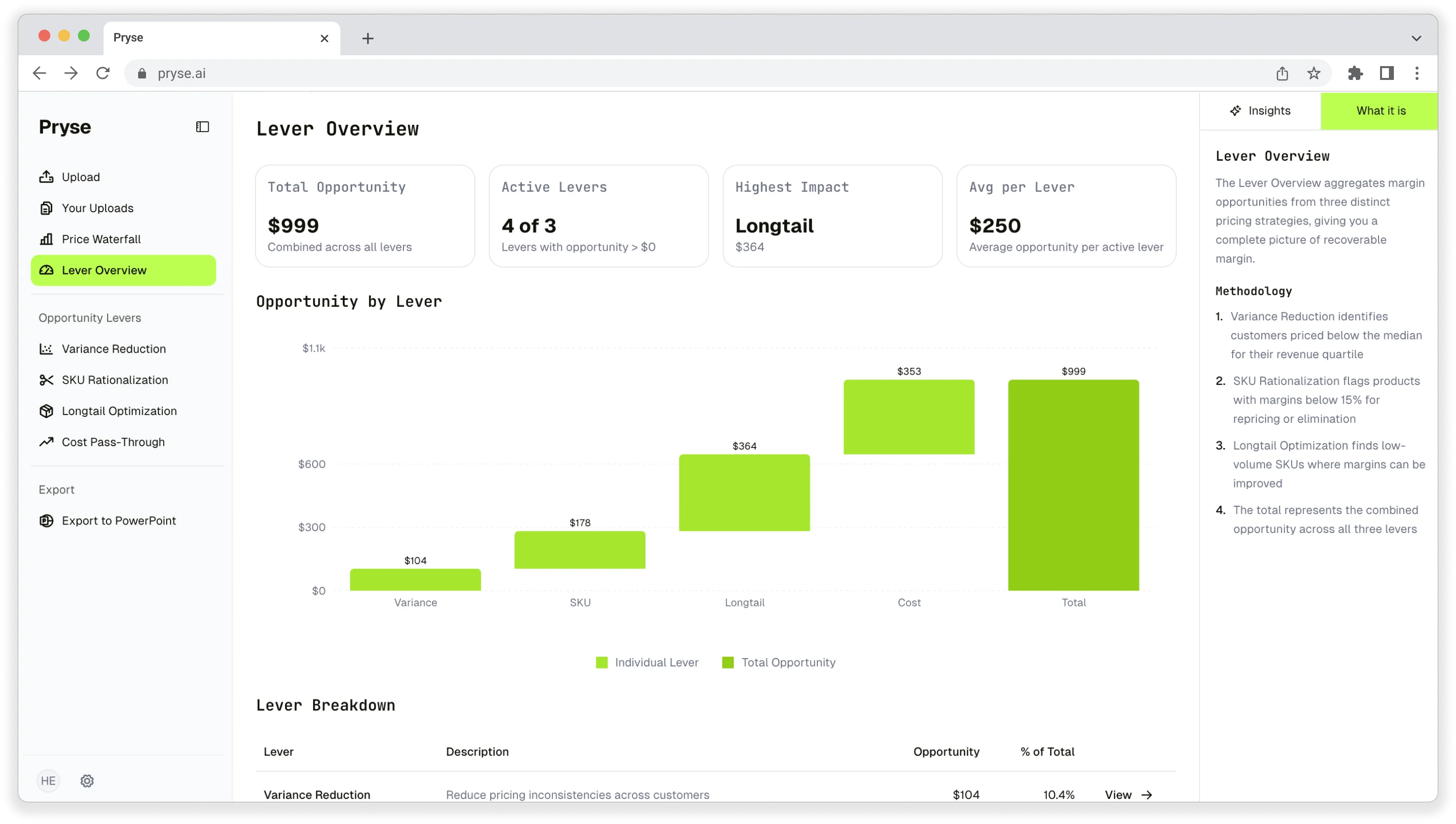
Pryse analyzes your transaction data to show where you're leaving money on the table. Upload your sales history and the tool identifies:
- Products priced below cost
- Customers getting inconsistent discounts
- Margin variation that signals pricing problems
- SKUs where small price adjustments could recover significant margin
You don't need to calculate elasticity for 50,000 SKUs. You need to know which 500 SKUs have the biggest margin recovery opportunity.
Next Steps
The midpoint formula is the standard method for calculating price elasticity when you have two data points. It eliminates the directional bias in the basic formula and produces consistent, defensible coefficients.
For more on price elasticity concepts and how elasticity fits into pricing strategy, see:
- Price Elasticity of Demand Formula — basic formula and interpretation
- Price Elasticity Calculator — tools and templates for elasticity calculation
- Price Elasticity Guide — complete framework for using elasticity in B2B pricing
If you want to identify pricing opportunities across thousands of SKUs without calculating elasticity coefficients, start with a margin diagnostic. Pryse analyzes your pricing data to find margin leakage and pricing inconsistencies in 24 hours.
Sources
- Calculating Price Elasticities Using the Midpoint Formula - Lumen Learning
- Arc Elasticity - Corporate Finance Institute
- Elasticity and the Midpoint Method - Pearson
- Midpoint Method in Economics - Economics Online
- Midpoint Formula: Definition, Uses & Examples - Outlier
- Arc Elasticity of Demand - Economics Help
Last updated: February 24, 2026
Frequently Asked Questions
Want to analyze your entire product catalog?
Pryse automatically identifies margin leakage across thousands of SKUs. Upload your data and find hidden profit in 24 hours.
One-time $1,499 diagnostic. No subscription required.