Price Elasticity of Supply: Formula, Calculation & What It Means for Pricing
Learn how price elasticity of supply measures producer responsiveness to price changes. Includes formula, calculation examples, and B2B manufacturing/distribution applications.
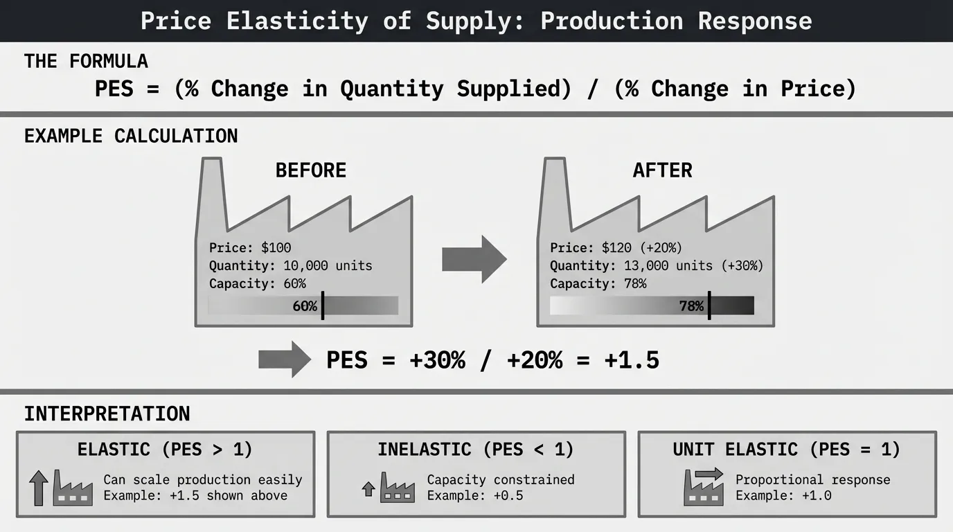
Price elasticity of supply measures how much quantity supplied changes when price changes. It's calculated as (% Change in Quantity Supplied) / (% Change in Price). A coefficient of +1.5 means a 10% price increase causes producers to supply 15% more product.
Unlike price elasticity of demand, which is always negative, supply elasticity is typically positive. When prices go up, suppliers produce more. When prices go down, suppliers produce less. That's the law of supply.
The coefficient tells you how much production capacity can flex in response to market prices. A manufacturer with elastic supply can ramp up production when prices rise. A manufacturer with inelastic supply is capacity-constrained and can't respond much to price signals.
The Price Elasticity of Supply Formula
According to Lumen Learning, price elasticity of supply is the percentage change in quantity supplied divided by the percentage change in price.
PES = (% Change in Quantity Supplied) / (% Change in Price)
Or with variables:
PES = ((Qs₂ - Qs₁) / Qs₁) / ((P₂ - P₁) / P₁)
Where:
Qs₁ = Original quantity supplied
Qs₂ = New quantity supplied
P₁ = Original price
P₂ = New price
The result is almost always positive because price and quantity supplied move in the same direction. When price goes up, quantity supplied goes up. When price goes down, quantity supplied goes down.
A coefficient greater than 1 means supply is elastic. Producers can respond strongly to price changes. A coefficient less than 1 means supply is inelastic. Production constraints limit how much suppliers can increase output.
Worked Example: Basic Formula
A fastener manufacturer produces 50,000 units per month of stainless steel bolts at $1.20 per unit. The market price increases to $1.50 per unit. They expand production to 65,000 units per month. What's the price elasticity of supply?
Step 1: Calculate percentage change in quantity supplied
(Qs₂ - Qs₁) / Qs₁ = (65,000 - 50,000) / 50,000 = 15,000 / 50,000 = 0.30 = 30%
Step 2: Calculate percentage change in price
(P₂ - P₁) / P₁ = (1.50 - 1.20) / 1.20 = 0.30 / 1.20 = 0.25 = 25%
Step 3: Divide quantity change by price change
PES = 30% / 25% = 1.20
The price elasticity of supply is +1.20. This product has elastic supply. A 1% price increase causes the manufacturer to produce 1.2% more. The manufacturer had spare production capacity and was able to respond to the higher price.
Revenue impact: Original revenue was $60,000/month (50,000 × $1.20). New revenue is $97,500/month (65,000 × $1.50). Revenue increased by $37,500 because the manufacturer could scale production to meet higher prices.
The Midpoint Method for Supply Elasticity
The basic formula has the same problem as demand elasticity. It gives different results depending on which direction you measure.
Say price increases from $100 to $120, and quantity supplied increases from 200 to 250 units. Then price falls back to $100, and quantity returns to 200. Using the basic formula:
- Price increase: 20% price change, 25% quantity change = elasticity of +1.25
- Price decrease: -16.7% price change, -20% quantity change = elasticity of +1.20
Same product. Same production response. Different elasticity coefficients. That's a measurement problem.
The midpoint method fixes this by using the average of starting and ending values. According to Khan Academy, the price elasticity of supply is calculated as the percentage change in quantity divided by the percentage change in price, and the midpoint method is a more accurate approach.
PES = ((Qs₂ - Qs₁) / ((Qs₁ + Qs₂) / 2)) / ((P₂ - P₁) / ((P₁ + P₂) / 2))
Simplified:
PES = ((Qs₂ - Qs₁) / (Qs₁ + Qs₂)) / ((P₂ - P₁) / (P₁ + P₂))
This produces the same elasticity coefficient whether you're measuring a price increase or price decrease between the same two points.
Worked Example: Midpoint Method
An electrical distributor supplies 12,000 breaker panels per quarter at $180 each. Market prices increase to $210. They increase supply to 14,400 panels. What's the supply elasticity using the midpoint method?
Step 1: Calculate the average quantity
Average Qs = (Qs₁ + Qs₂) / 2 = (12,000 + 14,400) / 2 = 13,200
Step 2: Calculate the average price
Average P = (P₁ + P₂) / 2 = (180 + 210) / 2 = 195
Step 3: Calculate percentage change in quantity using the average
% Change Qs = (Qs₂ - Qs₁) / Average Qs = (14,400 - 12,000) / 13,200 = 2,400 / 13,200 = 0.182 = 18.2%
Step 4: Calculate percentage change in price using the average
% Change P = (P₂ - P₁) / Average P = (210 - 180) / 195 = 30 / 195 = 0.154 = 15.4%
Step 5: Divide
PES = 18.2% / 15.4% = 1.18
The price elasticity of supply is +1.18 using the midpoint method. If you reverse the calculation (starting from $210 and dropping to $180), you get the same coefficient. That's the advantage.
Revenue check: Original revenue was $2,160,000/quarter (12,000 × $180). New revenue is $3,024,000/quarter (14,400 × $210). The distributor captured higher prices and increased volume, because their supply was elastic enough to respond.
Interpreting the Results: Elastic vs Inelastic Supply
The coefficient tells you how responsive production is to price changes. According to OpenStax, if elasticity is greater than one, the supply is elastic; if less than one, supply is inelastic.
| Coefficient | Interpretation | What It Means for Production |
|---|---|---|
| 0 | Perfectly inelastic | Quantity supplied doesn't respond to price. Fixed capacity, no ability to scale. |
| 0 to 1 | Inelastic | Producers are constrained. Price increases generate modest production increases. Limited spare capacity. |
| Exactly 1 | Unit elastic | Price and quantity changes are proportional. 10% price increase = 10% production increase. |
| Greater than 1 | Elastic | Producers can scale production easily. Price increases generate strong production responses. Spare capacity available. |
| Infinite | Perfectly elastic | Producers will supply any quantity at the current price. Horizontal supply curve. |
The higher the coefficient, the more elastic the supply. A coefficient of +2.5 means production responds more strongly to price changes than a coefficient of +0.8.
Examples by category:
-
Agricultural products (short run): Highly inelastic (+0.1 to +0.4). You can't grow more wheat overnight. Production cycles are long, and you can't speed up biology.
-
Manufacturing with spare capacity: Elastic (+1.2 to +2.5). Factories with unused production lines can add shifts, hire workers, and scale output quickly when prices rise.
-
Manufacturing at full capacity: Inelastic (+0.3 to +0.7). Factories running 24/7 can't increase output much without building new facilities or buying more equipment. That takes time and capital.
-
Specialty manufacturing with custom equipment: Highly inelastic (+0.1 to +0.5). Custom production requires specialized tooling, trained workers, and long lead times. Price increases don't immediately translate to higher output.
-
Simple assembly or commoditized production: Highly elastic (+2.0 to +5.0). Products like phone accessories, basic textiles, or mass-produced consumer goods can scale production rapidly because equipment and labor are readily available.
Price Elasticity of Supply in the Short Run vs Long Run
According to Economics Help, supply is normally more elastic in the long run than in the short run for produced goods, since in the long run all factors of production can be utilized to increase supply.
In the short run, at least one factor of production is fixed. A manufacturer has a fixed number of machines, a fixed factory size, and a fixed workforce trained on those machines. They can add overtime shifts or run equipment harder, but they can't dramatically increase output. Supply is inelastic.
In the long run, all factors are variable. The manufacturer can build a second factory, buy more equipment, hire and train more workers, and negotiate long-term contracts for raw materials. Production capacity can expand significantly. Supply becomes elastic.
Short-run constraints that make supply inelastic:
- Fixed production capacity (machines, factory floor space)
- Existing workforce with fixed skills
- Long lead times for equipment or raw materials
- Inventory limitations
Long-run adjustments that make supply elastic:
- Build new facilities or expand existing ones
- Purchase additional equipment
- Hire and train new workers
- Develop new suppliers or negotiate better terms
- Improve production efficiency through process optimization
Example: Electrical distributor
Short run (1-3 months): A distributor can't significantly increase supply. Their warehouse space, delivery trucks, and supplier contracts are fixed. If breaker panel prices increase 20%, they might increase supply 5% by working weekends and pushing suppliers for faster delivery. PES = +0.25 (inelastic).
Long run (12-24 months): The distributor can lease a larger warehouse, hire more delivery drivers, buy more trucks, and negotiate contracts with additional suppliers. A 20% price increase might lead to a 40% supply increase. PES = +2.0 (elastic).
What Makes Supply Elastic or Inelastic?
According to Marshall Education, the greater the extent of spare production capacity, the quicker suppliers can respond to price changes and hence the more price elastic the supply would be.
Factors that make supply elastic (PES > 1):
-
Spare production capacity. Factories running at 60% utilization can add shifts and scale output quickly. A producer with unused capacity can quickly respond to price changes, assuming variable factors are readily available.
-
Readily available inputs. If raw materials, labor, and equipment are easy to source, production can scale. Commodity inputs with multiple suppliers support elastic supply.
-
Simple production processes. Products that don't require specialized skills, custom tooling, or long assembly times can scale faster. A clothing manufacturer can hire workers and increase production relatively quickly.
-
Low capital intensity. Businesses that don't require expensive equipment or large facilities can enter or exit markets quickly. Service businesses often have elastic supply because they just need to hire people.
-
Long time horizon. Given enough time, nearly all supply becomes elastic. Producers can build new facilities, develop new suppliers, and train workers.
Factors that make supply inelastic (PES < 1):
-
Full capacity utilization. According to Marshall Education, as capacity becomes fully utilized, increasing production requires additional investment in capital (like plant and equipment). Since price must rise substantially to cover this expense, supply becomes less elastic at high output levels.
-
Scarce or specialized inputs. If production requires rare materials, specialized equipment, or highly trained workers, scaling is difficult. Diamond mining has inelastic supply because new mines take years to develop.
-
Long production cycles. Agricultural products have inelastic short-run supply because crops take months to grow. You can't plant wheat in March and harvest it in April just because prices went up.
-
Regulatory barriers. Industries with licensing requirements, environmental regulations, or safety certifications can't scale quickly. Pharmaceutical manufacturing is inelastic because building a new FDA-approved facility takes years.
-
High capital requirements. Building new factories, buying specialized equipment, or developing infrastructure takes time and money. Steel production has inelastic supply because blast furnaces cost hundreds of millions of dollars and take years to build.
Price Elasticity of Supply vs Price Elasticity of Demand
Both measure responsiveness to price changes, but they measure different sides of the market. According to Khan Academy, the price elasticity of demand is the percentage change in quantity demanded divided by the percentage change in price, while the price elasticity of supply is the percentage change in quantity supplied divided by the percentage change in price.
| Dimension | Price Elasticity of Demand | Price Elasticity of Supply |
|---|---|---|
| What it measures | Consumer responsiveness to price | Producer responsiveness to price |
| Sign | Always negative (price and quantity move opposite) | Typically positive (price and quantity move together) |
| Formula | (% ΔQd) / (% ΔP) | (% ΔQs) / (% ΔP) |
| Interpretation | How much volume you lose from price increases | How much production capacity you can add when prices rise |
| Elastic means | Coefficient < -1 (e.g., -2.5) | Coefficient > +1 (e.g., +2.5) |
| Inelastic means | Coefficient between 0 and -1 (e.g., -0.4) | Coefficient between 0 and +1 (e.g., +0.4) |
| Use case | Pricing decisions: will a price increase hurt revenue? | Production planning: can we meet higher demand? |
Both concepts use the same threshold of 1 for elasticity categories. Corporate Finance Institute confirms that elasticities greater than one indicate high responsiveness (elastic), while elasticities less than one indicate low responsiveness (inelastic).
You need both to make smart pricing and production decisions. Demand elasticity tells you how customers will respond to price changes. Supply elasticity tells you whether you can actually deliver more product if demand increases.
Price Elasticity of Supply in B2B Markets
Most elasticity examples use consumer goods. Manufacturing and distribution markets behave differently.
1. Supply constraints vary by customer segment. Large OEM customers often require long-term supply agreements with minimum capacity commitments. Small customers buy spot market quantities. The same manufacturer might have inelastic supply for large customers (capacity is pre-allocated) and elastic supply for small customers (they can flex spot production).
2. Switching costs affect supply response. In consumer markets, producers can sell to different customers easily. In B2B, customers have qualification requirements, testing protocols, and approved vendor lists. A manufacturer can't just redirect supply from Customer A to Customer B when Customer B offers a higher price. Switching costs make supply less elastic than the production capacity suggests.
3. Contract pricing locks in supply. If 70% of a manufacturer's capacity is committed to 12-month contracts at fixed prices, supply elasticity on the remaining 30% is what matters for short-term price signals. The manufacturer might have elastic production capacity overall but inelastic uncommitted capacity.
4. Production planning cycles create lags. Consumer goods manufacturers can adjust production weekly or monthly. B2B manufacturers often plan production quarters in advance based on customer forecasts. A price increase in February might not affect production until the next planning cycle in April. Supply elasticity depends on planning cycles, not just physical capacity.
5. Capital intensity matters more. B2B manufacturing often requires expensive, specialized equipment. A machine shop can't add CNC machines overnight when prices rise. An electrical distributor can add warehouse space and trucks relatively quickly. Capital-light distribution has more elastic supply than capital-intensive manufacturing.
When Not to Trust the Supply Elasticity Coefficient
Supply elasticity formulas assume rational production decisions and flexible capacity. Real markets sometimes break those assumptions.
Regulatory constraints. If production requires permits, environmental reviews, or safety certifications, supply is inelastic regardless of physical capacity. A pharmaceutical manufacturer might have spare capacity but can't increase production without FDA approval, which takes months.
Supply chain dependencies. A manufacturer might be able to scale assembly quickly, but if a critical component comes from a single supplier with long lead times, supply is inelastic. The bottleneck determines elasticity, not internal capacity.
Seasonal products. Agricultural products have highly inelastic supply within a growing season. Wheat farmers can't grow more wheat in July just because prices went up. But they can plant more acres next season, making long-run supply elastic.
Peak capacity limits. A distributor might have elastic supply at normal volume levels but inelastic supply at peak levels. During seasonal demand spikes, warehouse space, delivery capacity, and workforce are fully utilized. Supply elasticity changes with utilization rates.
Economic cycles. During recessions, manufacturers have spare capacity and elastic supply. During booms, factories run at full capacity and supply becomes inelastic. Elasticity coefficients measured in 2020 might not apply in 2024.
Calculating Supply Elasticity with Transaction Data
Most mid-market companies can calculate supply elasticity in Excel if they have production and pricing data.
What you need:
- Production history with at least 12 months of data
- Columns for: Date, Product, Quantity Produced, Price Received
- Price variation over time (if your prices never change, you can't measure elasticity)
Steps:
- Segment data by product or product category
- Group by month or quarter
- Calculate average price and total quantity produced for each period
- Apply the midpoint formula between consecutive periods
- Average the elasticity coefficients to get a product-level estimate
This won't be as precise as econometric analysis, but it's enough to identify which products have elastic supply (you can scale production easily) vs inelastic supply (capacity-constrained).
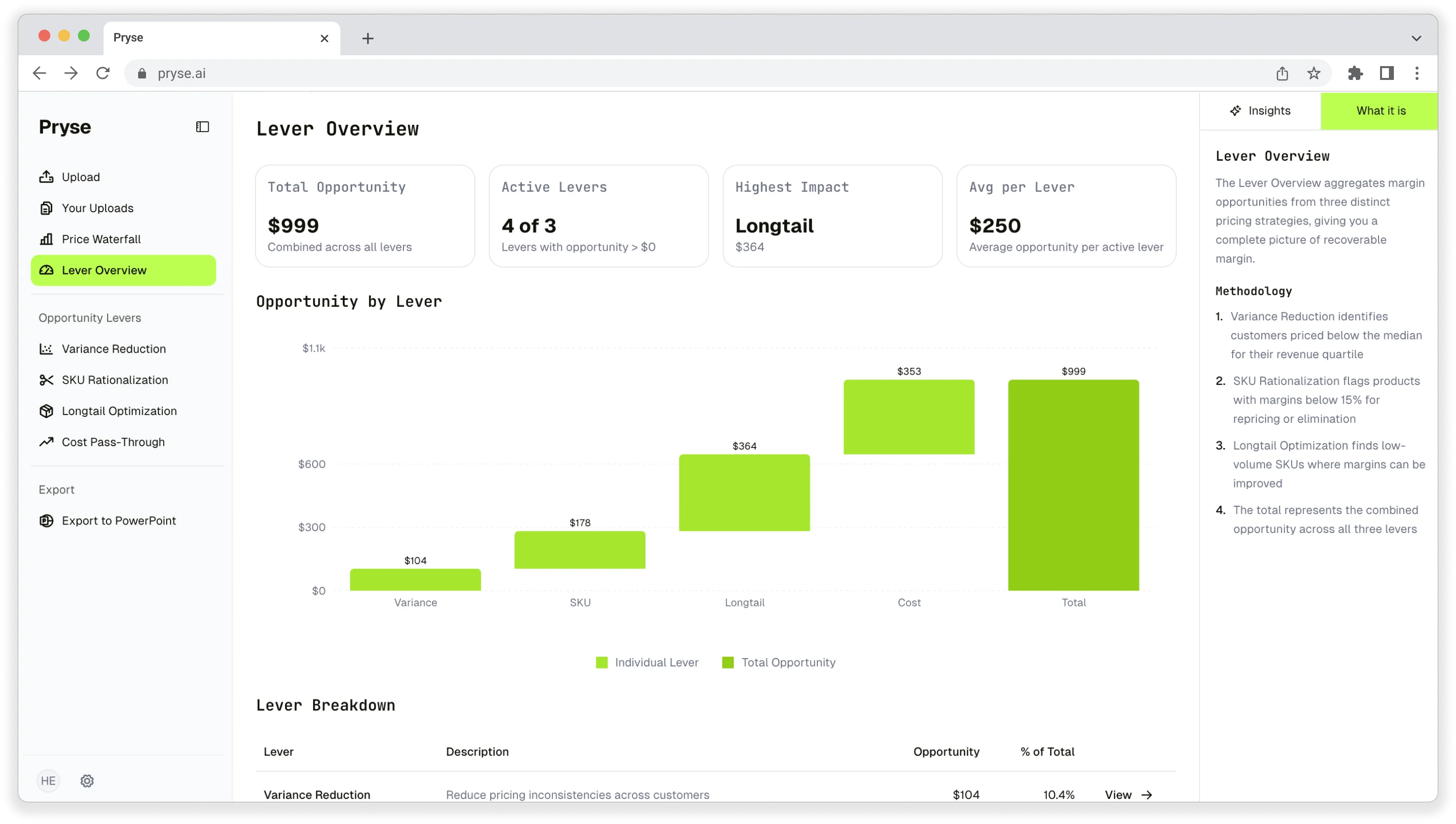
For companies managing thousands of SKUs, understanding pricing capacity tradeoffs is critical. Pryse's margin diagnostic analyzes transaction data to identify margin leakage and pricing opportunities across your product catalog. You upload your ERP data, and the tool shows where pricing doesn't match realized margins.
What to Do With Your Supply Elasticity Coefficient
Calculating elasticity is useful. Acting on it is where the value is.
If your supply is elastic (coefficient > 1):
- You can capture market share by scaling production when competitors can't
- Respond aggressively to price increases—you won't leave demand unmet
- Focus on sales and marketing to drive volume—production can keep up
- Consider volume-based pricing strategies that reward customers for larger orders
If your supply is inelastic (coefficient < 1):
- You can't scale production quickly, so focus on margin, not volume
- Raise prices during high-demand periods—you're capacity-constrained anyway
- Don't over-promise lead times or delivery quantities
- Invest in capacity expansion if high prices are sustainable
- Use allocation strategies to prioritize high-margin customers or products
If your supply is unit elastic (coefficient near 1):
- Production scales proportionally with price signals
- Balance volume and margin goals—neither dominates
- Plan capacity investments based on price trends
- Monitor competitors' capacity to understand market supply elasticity
Practical Applications for Manufacturers and Distributors
For manufacturers:
-
Capacity planning. If your supply is elastic, you can afford to pursue aggressive volume growth. If your supply is inelastic, focus on margin and be selective about which customers and products you prioritize.
-
Pricing strategy. Manufacturers with inelastic supply should use value-based pricing and capture margin. Manufacturers with elastic supply can use competitive pricing to win share because they can fulfill the volume.
-
Contract negotiations. If a customer wants guaranteed capacity at fixed prices, charge more when your supply is inelastic. You're giving up the option to sell to higher-paying customers when demand spikes.
For distributors:
-
Inventory management. Distributors have elastic supply for most products (they buy from manufacturers, not produce). But warehouse space and working capital create constraints. Measure supply elasticity for your top-selling categories to understand how much you can scale.
-
Supplier relationships. Know which suppliers have elastic supply (can deliver more when you need it) vs inelastic supply (capacity-constrained). Diversify your supplier base for inelastic categories to avoid stockouts.
-
Dynamic pricing. If your supply is elastic, you can run promotions and drive volume without worrying about fulfillment. If your supply is inelastic (limited warehouse space or capital), use higher prices to ration inventory to the highest-margin customers.
Common Mistakes When Calculating Supply Elasticity
Mistake 1: Confusing production capacity with supply. Capacity measures maximum output. Supply measures willingness to produce at a given price. A manufacturer with 50% spare capacity might still have inelastic supply if raw materials are expensive or uncertain. Capacity is a physical constraint. Supply is an economic decision.
Mistake 2: Ignoring time horizons. Supply elasticity changes with time. Short-run supply might be inelastic (fixed capacity), while long-run supply is elastic (can build more capacity). Always specify the time frame when calculating elasticity.
Mistake 3: Treating supply as constant. Supply elasticity changes as you move up or down the supply curve. At low production levels, supply is elastic (lots of spare capacity). At high production levels, supply becomes inelastic (approaching capacity limits). Your elasticity coefficient is only valid near the current production level.
Mistake 4: Using average costs instead of marginal costs. Supply decisions are based on marginal cost, not average cost. A manufacturer with high fixed costs might appear to have inelastic supply using average cost analysis, but elastic supply when considering only marginal costs of producing one more unit.
Mistake 5: Ignoring external constraints. Supply elasticity isn't just about your factory. It's about your suppliers, workforce availability, regulatory approvals, and logistics capacity. A bottleneck anywhere in the supply chain makes overall supply inelastic.
When to Use Each Formula
Use the basic formula when:
- You're forecasting production response to future price changes
- You're working with small price adjustments (under 5%)
- You need a quick directional answer for capacity planning
Use the midpoint method when:
- You're analyzing historical data to measure what happened
- You're comparing supply elasticity across different products or facilities
- You need precision for larger price or volume changes
- You're presenting analysis to executives or boards
The midpoint method is more accurate for analysis. The basic formula is faster for estimation. For small price changes (2-3%), both formulas give similar results. The gap widens for large changes.
Next Steps
Supply elasticity tells you how quickly you can scale production when prices rise. It's a production planning metric as much as a pricing metric. For manufacturers, it determines whether to compete on volume or margin. For distributors, it determines how aggressively to pursue volume growth.
For more on using elasticity in your pricing strategy, see our complete Price Elasticity Guide. To understand how demand responds to price changes, start with Price Elasticity of Demand Formula.
If you want to identify pricing opportunities and margin leakage across your product catalog without calculating elasticity for every SKU, start with a transaction analysis. Pryse analyzes your pricing data to show where you're leaving money on the table—no elasticity calculations required.
Sources
- Price Elasticity of Supply - Lumen Learning
- Price Elasticity of Demand and Price Elasticity of Supply - Khan Academy
- Price Elasticity of Supply - Economics Help
- Price Elasticity of Demand and Supply - OpenStax
- Determinants of Price Elasticity of Supply - Marshall Education
- Price Elasticity - Corporate Finance Institute
- Price Elasticity of Supply (Wikipedia)
Last updated: February 24, 2026
Frequently Asked Questions
Want to analyze your entire product catalog?
Pryse automatically identifies margin leakage across thousands of SKUs. Upload your data and find hidden profit in 24 hours.
One-time $1,499 diagnostic. No subscription required.